An Approach towards Optimizing Random Forest using Dynamic Programming Algorithm

An Approach towards Optimizing Random Forest using

Dynamic Programming Algorithm

Vrushali Y Kulkarni

COEP, Pune, India

Aashu Singh

MIT Pune, India

Pradeep K Sinha CDAC, Pune, India

ABSTRACT

Random Forest (RF) is an ensemble supervised machine learning technique. Based on bagging and random feature selection, number of decision trees (base classifiers) is generated and majority voting is taken among them. The size of RF is subjective and varies from one dataset to another. Furthermore due to the randomization induced during creation, and its huge size, RF has at best been described as black-box. Various changes based on the experimental results have been proposed in the algorithm since then to optimize the performance of RF. To this end, we aim to find a subset, having accuracy comparable to original RF but having a much smaller size. In this paper, we show that the problem of selection of optimal subset of random forest follows the dynamic programming paradigm. Applying this approach to various UCI data-sets, corresponding subsets are obtained and studied. We conclude that such subsets do exist and that they are not unique. Moreover the size of these subsets is small fraction of the original RF (in the range of tens) and that accuracy of these subsets is a discrete valued function over its range.

General Terms

Data Mining, Machine Learning

Keywords

Ensemble classifier, Random Forest, Decision tree, Dynamic Programming, Optimal subset

1.

INTRODUCTION

Random forest belongs to the family of classifier ensemble methods that use randomization to produce a diverse pool of individual classifiers. It can be defined as a classifier consisting of a collection of L tree-structured classifier {h(x, Θ k), k = 1. . . L} where the {Θ k} are independent identically

distributed random vectors and each tree casts a unit vote for the most popular class at input x [1]. A random forest can be built by randomly sampling a feature set for each decision tree (as in Random Subspaces [2]), and/or by random sampling a training subset for each decision tree (as in Bagging [3]). Random Forest (RF) has emerged as one of the most commonly used classification methods. Several characteristics that make it ideal are: It can be used when there are many more variables than observations, It has good predictive performance even when most predictive variables are noise, It does not over-fit, It can handle a mixture of categorical and continuous predictors.

A major drawback of RF is that it is virtually impractical to interpret the forest. This can be attributed in part to large number of trees grown in the original forest along with

[1] referred to them as ‘Black Box’. This provided the impetus for our work towards understanding the various aspects of RF performance. Several experiments by Simon Bernard et al, [4][5], have shown that suboptimal subsets of RF do exist and that they have better accuracy than the entire forest. Zhang and Wang [6] have demonstrated the existence of an optimal subset for the Breast Cancer dataset. In this paper, we use the Dynamic programming algorithm to obtain optimal subset of the random forest. Simulating the experiment on various datasets from UCI repository, we obtain the corresponding optimal subsets. We show that these optimal sets are not unique and that a significant number of subsets have higher accuracy as compared to the original RF. This paper is organized in following way: Section 2 introduces Random Forest Algorithm and some recent work in the area. Section 3 introduces dynamic programming approach and its application in obtaining optimal subset. Section 4 and 5 describe the experiments conducted and discuss the results at length. Section 6 gives concluding remarks.

2.

CURRENT SENARIO

The Forest-RI algorithm [1] by Breiman is often cited as the reference algorithm in the literature. It uses the concept of Bagging with another randomization technique called Random Feature Selection. The training step creates an ensemble of decision trees, each one trained from a bootstrap sample of the original training set created through bagging and a decision tree induction method. In this induction algorithm, a subset of feature is drawn randomly and the best splitting criterion is selected at each node.

The Forest-RI method can be summarized by the following steps:

-Let N be the size of the original training set. N

instances are drawn at random with replacement, to form a bootstrap sample, which is then used to build a tree.

-Let M be the total number of attributes and K be the fixed parameter such that K∈ [1..M]. At each node of the tree, a subset of K (K<<M) features is randomly selected without replacement. The best split among them is then selected.

-The tree is thus built to its maximum size. No pruning is performed.

Such ensemble of Random Trees constitutes Random Forest.

demonstrated that performance of random forest is improved in some domains by replacing majority voting with Dynamic Integration, which is based on local prediction performances of base decision trees. Robnik and Sikonja [9] have shown that Weighted Voting with RF has better performance. In their work, Tripoliti, Fotiadis, and Manis [10] determine the number of decision trees in random forest during the growing procedure of forest. The method is based on on-line curve fitting. The forest construction first starts with 10 trees. During each iteration a new tree is added and tested if it is a best fit. Some heuristics based changes like selective attribute and bootstrap sample selection for generation of base classifiers have been shown to give improved performance [11]. Many of the tasks in data mining domain concern high-dimensional data. Consequently, these tasks are often complex and computationally expensive. A GPU-based implementation of Random Forest algorithm is developed, which is based on Compute Unified Device Architecture (CUDA). The algorithm is experimentally evaluated on NVIDIA GT 220 graphics card with 48 CUDA cores and 1 GB of memory. Both training phase and classification phase are parallelized in CUDA implementation. CudaRF outperforms both LibRF and FastRF in Weka [12] for specified classification task [13]. Online Random forest algorithm [14] generates on-line decision trees based on concepts from on-line bagging and extremely randomized forests. It also uses Temporal Weighting scheme to discard non performing trees based on their out-of-bag error performance. The algorithm is ported onto NVIDIA GPU which has shown ten times speed up. Incremental Extremely Random forest algorithm is specially designed for small data streams [15]. The algorithm works on the basis of expanding the leaf nodes without reconstructing the whole trees. Random Forest has shown good results for imbalanced data [16], and problems of large P small n paradigm [17]. Fuzzy Random Forest [18] and Random Forest using semi supervised learning approach [19] are also being targeted by the researchers. We have done systematic survey of Random Forest classifiers in [22].

Breiman [1] stated that RF does not over-fit, that is as number of trees are added to the forest, generalization error (PE*) attains a maximum value. In other words, beyond a certain point, addition of more trees does not lead to increase in accuracy. The work of Latinne et al. in [20] and Simon Bernard et al. in [4] experimentally confirms this statement. The idea of our experimental work is to establish how well a subset of RF is able to outperform the original ensemble and whether such performance improvements are observed over wide range of datasets.

3.

DYNAMIC PROGRAMMING

3.1

Introduction

Dynamic Programming is an algorithm design method that can be used when the solution to a problem can be viewed as the result of sequence of decisions. It solves problems by combining solutions to sub-problems. It is applicable when the problems are not independent, that is, when sub-problems share sub-sub-problems [21]. A Dynamic Programming algorithm solves every sub-sub-problem just once and then saves its answer in a table, thereby avoiding the work of re-computing the answer every time the sub-problem is encountered.

The two key ingredients that an optimization problem must have in order for dynamic programming to be applicable are: 1.) Optimal Substructure: A problem exhibits optimal substructure if an optimal solution to the problem contains within it, optimal solution to sub-problems.

2.) Overlapping Sub-problems: When a recursive algorithm revisits the same problem over and over again, it is said that optimization problem has overlapping sub-problems.

3.2

Applicability

The problem of finding an optimal subset of RF should exhibit the above mentioned properties, for the applicability of Dynamic Programming. The objective function for identifying the optimality of the set has been taken as its accuracy.

Optimal Substructure: Suppose we have a RF of n trees namely T1,T2,...,Tn. Finding an optimal subset of size k entails

finding an optimal subset of size k-1. For if the subset of size k-1 is not optimal, than we can substitute a more optimal subset of size k-1 to yield a more optimal subset of size k, a contradiction.

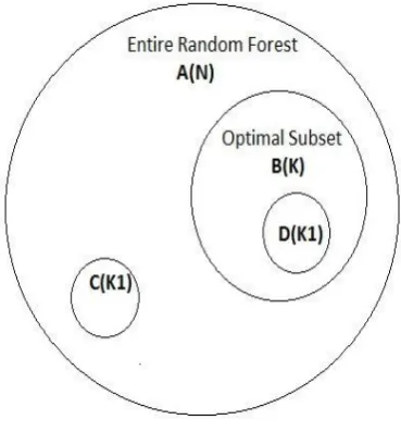
This property states that any subset of optimal set would be optimal among all the subsets of its size, the subset belonging to optimal set would have highest accuracy.

Fig 1: Subsets of Random Forest

In Figure1, A(N) represents the entire forest of size N and B(K) represents an optimal subset of size K. Following the Optimal Substructure property, C(K1) and D(K1) are subsets of size K1 where K>K1. ‘D’ has the highest accuracy among all the subsets of size K1.

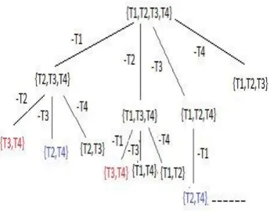
Overlapping Sub-problems: Let us assume, we have a RF containing 4 elements namely T1,T2,T3 and T4. Now to choose

Fig 2: Similarly colored subsets represent overlapping sub-problems

Consider Figure 2, in each iteration one tree of the forest is eliminated. The cost of computing accuracy of the subset obtained after removing trees T1 then T2 is same as that

obtained by first removing T2 and then T1. In this process of

finding the optimal subset, many subsets of RF re-appear. The overlapping sub-problems have been marked with same color. We store the accuracy for each of the distinct subsets and later when the subsets re-appear, values can be simply looked up. In this way problem of finding optimal subset of RF has been modeled using Dynamic Programming. As can be seen from the Figure 2, at each stage the number of unique subsets obtained by removing trees can be expressed as NCK where K is the size of subsets at that stage. Thus total

number of distinct subsets can be shown as

using the formula for binomial expansion. A close look at the expression reveals that we have in fact enumerated Power-Set of size N (2N). The two subsets left out are empty set which is of no use and complete set which represents the original RF. We present the algorithm for finding the optimal subset as follows:

3.3

Time Complexity

The algorithm requires one to iterate through power-Set of size N. Assuming a constant time for generating the subset Si

and calculating Ai since these hardly vary with size of subset.

So time complexity is O =O (

3.4

Space Complexity

In order to avoid huge memory requirements for storing power-set we use the algorithm based on binary counter for enumerating subsets one at a time. The subsets are evaluated simultaneously and those with favorable results are stored back onto the disk in the form of text-file. Space requirements vary linearly with the size of subset due to the number of trees contained in the set. Maximum space requirement while running turns out to be O (N) + c. Hence the space complexity

Since there are no further constraints like minimum number of trees that need to be in the forest, our solution to the most optimal subset ends with selecting the subset with highest accuracy.

3.5

Experimental Protocol

Algorithm to find optimal subset of Random Forest

Input: N: Trees in the original forest.

Input: M: Features in the original dataset.

Input: I : Number of Instances in the original dataset.

Output Si’: Optimal Subset.

Parameters:

A: % Accuracy of original RF Si: ith subset.

Ai:%Accuracy obtained from subset Si

n(Si) : number of elements in Si / Size of Si

max-Accuracy: maximum accuracy recorded. min-Size: minimum size of Si

Method:

1. Set max-Accuracy and min-Size to arbitrarily large values outside the experimental range. max-Accuracy = 100%

min-Size = 1000

2. Calculate accuracy of original RF i.e. A. 3. Calculate P(N) : Power Set of N elements. 4. for i = 1 to P(N) {

5. Calculate accuracy of subset Si i.e. Ai

6. if (Ai >A) or (Ai = A and n(Si) < N){

7. Store Si.

8. if ((max-Accuracy < Ai ) ||

(max- Accuracy = = Ai and min-Size > n(Si))

9. Si’ = Si

10. max-Accuracy=Ai

11. min-Size = n(Si) }

12. Output Si’.

4.

METHODS AND RESULTS

Experiments have been performed in Java using Weka machine learning library. Since the time-complexity is

O(2N_{) the size of RF (i.e. N) is taken to be 15 to keep}

Mathematically, it can be expressed as: (Ai > A) || ((Ai = A) && Size (Si) < Size (RF))

Size – function to find number of elements in subset Si or

original Random Forest RF

The collection of subsets thus obtained, also includes optimal subset. Though one might feel that size of RF is too small to arrive at any practical conclusion about Random Forest in general, the results indeed show otherwise. With parallel RF implementation and more processing power, value of N can be increased.

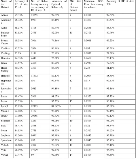
The datasets used for experimentation have been taken from UCI Machine Learning repository. The results of the experimentation for 33 datasets have been summarized in the form of table. It contains accuracy of original RF, and that of its corresponding optimal subsets. Furthermore the minimum size for each optimal subset is presented. It also lists the number of sub-optimal subsets having accuracy greater than original RF. Finally we table the accuracy of RF of size 300 to give an idea regarding how well the optimal subset fares in comparison to RF of sizes normally used for these data-sets. A quick glance at Table 1 reveals that large number of subsets have greater accuracy compared to the original RF. We delve into the details later.

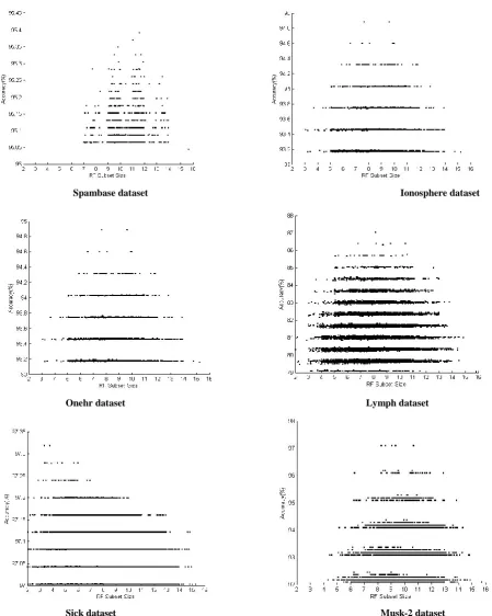
Figure 3 shows plots of subset accuracy vs. subset size. Only subsets having accuracy greater than or equal to original RF have been plotted. In order that accuracy plots of two subsets of same size do not overlap each other, it has been distributed randomly in the range between current subset size and next higher one. Eg. Accuracy measure corresponding to subset of size S is plotted in the range [S, S+1). It can be observed that there are multiple subsets of different sizes having accuracy higher than the original RF of size 15 and that many of these have same accuracy. The size of these subsets varies from one dataset to another. The optimal subset among these is the one with the highest accuracy. In some datasets, as in the case of Letter, there are no subsets having accuracy greater than original RF. This simply means that learning is insufficient and that more number of trees is required in the forest. Moving ahead Figure 4 shows 3D plot of these subsets. On X-axis size of the sub-Forest is plotted, on Y-X-axis its corresponding accuracy in percentage and on Z-axis its corresponding OOB error rate. Now as seen in the experimentation the optimal subset – one with highest accuracy need not necessarily have the lowest OOB Error rate. OOB error rate indicates the ability of the set to generalize - lower the OOB error rate better is the generalization. Accordingly depending on the requirement the subset can be chosen satisfying the accuracy and

generalization requirements. Such region containing various optimal and sub-optimal subsets can be identified easily in the 3D plot. It is the one surrounding the point where all the red lines meet; here accuracy is maximum while OOB error rate is minimum. Choosing a set from this region would give us ideal subset – one which not only gives better performance but also generalizes well.

A keen observation of Figure 3 reveals that accuracy of subsets take discrete values. This can be gauged from the fact that accuracy does not vary continuously over its entire range, rather it takes some discrete values and that these values differ from one dataset to another. The accuracy points when plotted on the graph form discrete bands. These discrete bands are thick (dense) and longer at the base meaning that large number of subsets over wide range of sizes have less accuracy. As accuracy increases, these bands become narrow and sparse indicating that few subsets have higher accuracy. Another important observation is that, subset with highest accuracy need not be unique as can be observed in graphs of Musk-2 and Sick. In these cases, the optimal subset is taken as one with least number of elements.

Finally in order to get an actual measure of performance of optimal subsets, we grow RF of size 300 and compare the performance. The results are recorded in the table. It can be seen clearly that in most of the cases, accuracy of optimal subset eclipses that of RF of size 300. Due to constraint in computing resources, size of RF for experimentation has been limited to 15. A larger size would give a more insight as regards the optimality and idealness of subsets. Since OOB error rate decreases exponentially with increase in subset size – as can be observed in Figure 4, study of Random Forests with size around 20 or 25 can give us subsets with better accuracy and generalization error rates.

5.

CONCLUSION

Table 1. Summary and Comparison of readings on various datasets

Name of the Dataset

Accuracy of RF of size 15 : A

No. of Subset having accuracy >= accuracy of RF of size 15.

Accuracy of Optimal Subset : Ai

Min Size of Optimal Subset

Minimum OOB Error Rate among the subsets

Accuracy of RF of Size 300

Anneal 99.33% 13355 99.89% 7 0.0314 99.67% Audiolog

y

78.32% 6923 83.18% 9 0.3269 80.53%

Autos 85.37% 1108 87.74% 9 0.2656 85.37%

Balance-Scale

81.12% 2441 82.09% 11 0.2103 80.96%

Breast-Cancer

69.58% 7966 74.16% 6 0.3061 69.23%

Credit-a 85.22% 3954 86.96% 8 0.193 85.51% Credit-g 75.2% 1118 76.80% 9 0.2872 77.30% Diabetes 74.35% 4440 76.31% 6 0.2669 75.13% Glass 77.57% 2478 80.90% 7 0.2923 77.57%

Heart-Statlog

80.74% 3399 83.70% 8 0.233 81.11%

Hepatitis 80.95% 11492 87.17% 6 0.2094 85.81% Hypothyr

oid

99.28% 959 99.44% 12 0.017 99.47%

Ionospher e

93.16% 3683 94.89% 7 0.1114 93.16%

Spambase dataset Ionosphere dataset

Sick dataset Musk-2 dataset

Spambase dataset Ionosphere dataset

Onehr dataset Sick dataset

Musk-2 dataset Lymph dataset

Fig.4. 3D plot of the sub-Forests for some of the datasets

X axis: Size of the sub-Forest (varies from 2 to 16).

6.

REFERENCES

[1] Leo Brieman, “Random Forests”, Machine Learning, 45, 5-32, (2001)

[2] Ho, T.: “The random subspace method for constructing decision forests” – IEEE Transactions on Pattern Analysis and Machine Intelligence (1998)

[3] Breiman, L.: “Bagging Predictors”–Machine Learning (1996)

[4] Simon Bernard, Laurent Heutte, and Sebastien Adam, “On the Selection of Decision Trees in Random Forest”, Proceedings of International Joint Cobference on Neural Networks, Atlanta, Georgia, USA, June 14-19, pp 302-307, (2009)

[5] Bernard, S., Heutte, L., Adam, S.: “Towards a Better Understanding of Random Forests Through the Study of Strength and Correlation” – 2009

[6] Heping Zhang, Minghui Wang, “Search for the smallest Random Forest”, Statistics and Its Interface Volume 2, pp 381-388, (2009)

[7] Boinee P, Angelis A and Foresti G, Meta Random Forest, International Journal of Computational Intelligence 2, (2006)

[8] Tsymbal A, Pechenizkiy M and Cunningham P, Dynamic Integration with Random Forest, ECML, LNAI, 801-808, Springer-Verlag (2006)

[9] Robnik M, Sikonja, Improving Random Forests, J F Boulicaut et al (eds): Machine Learning, ECML 2004 Proceedings, Springer, Berlin, (2004)

[10] E Tripoli, D Fotiadis, G Manis, “ Dynamic Construction of Random Forests: Evaluation using Biomedical Engineering Problems”, IEEE 2010

[11] Vrushali Kulkarni, Pradeep Sinha, Aashu Singh,: Heuristic Based Improvements for Effective Random Forest Classifier, Proceedings of International Conference on Computational Intelligence (published by Springer), Chennai, India, 2012

[12] I. H. Witten, E. Frank, Weka : Practical machine learning tools and techniques, Morgan Kaufmann publisher, (2005)

[13] Grahn H, Lavesson N, Lapajne M and Slat D, A CUDA implementation of Random Forest Early Results, Master Thesis Software Engineering,School of Computing, Blekinge Institute of Technology, Sweden

[14] Saffari A, Leistner C, Santner J, Godec M and Bischof H, On-line Random Forests, ICCV IEEE, Conference Proceedings 1393-1400, (2009)

[15] Wang A, Wan G, Cheng Z and Li S, An Incremental Extremely Random Forest Classifier for Online Learning and Tracking, 16th IEEE International Conference on Image Processing,1449-1452, (2009)

[16] Chain C, Liaw A and Breiman L, Using Random forest to Learn Imbalanced Data, Technical Report, Department of Statistics, U. C. Berkley (2004)

[17] Kosorok M and Ma S, Marginal Asymptotics for the Large p Small n paradigm: With Applications to Microarray Data, Ann Statist 35, 1456-1486, (2007) [18] Bonissone P, Cadenas J, Garrido M and Diaz-Valladares

R, A Fuzzy Random Forest, International Journal of Approximate Reasoning, 51, 729-747, (2010)

[19] Leistner C, Saffari A, Santner J, Godec M and Bischof H, Semi- Supervised Random Forests, ICCV IEEE, Conference Proceedings, 506-513 (2009)

[20] Patrice, L., Olivier, D., Christine, D.: “Limiting the Number of Trees in Random Forests” – 2nd International Workshop on Multiple Classifier Systems – MCS, Cambridge, UK (2001)

[21] Cormen, T., Leiserson, C., Rivest, R., Stein, C.: “Introduction To Algorithms” – 2nd _Edition.