Dynamic Wavelet Thresholding based Image Restoration

Dynamic Wavelet Thresholding based Image Restoration

Poonam Baruah

Amity School of Engineering and Technology, Amity University, Noida, India

ABSTRACT

Images are corrupted by various means during its acquisition, processing, compression, transmission and reproduction. However, a host of techniques are available which have explored many ways and means to improve the quality of restoration. The paper presents the restoration of an image by de-noising based on soft thresholding. The process recovers the degraded images by adapting a dynamic wavelet transform to minimize the error to an extent which helps in achieving satisfactory, quality and suitable forms for certain medical applications.

Keywords

Dynamic wavelet thresholding, image de-noising, image restoration, PSNR, MSE.

1. INTRODUCTION

Images corrupted by noise and other related degradations are required to be restored for their further processing. Such situations are often observed in various medical applications and satellite imaging. The goal of de-noising is to remove or suppress the noise while retaining the important features of the image as much as possible [1]. Wavelet analysis has been demonstrated to be one of the powerful methods for removal of image noise. Wavelet de-noising removes the noise present in the signal or image while preserving the original characteristics, regardless of its frequency content. However, wavelet de-noising is different from smoothing as it removes the high frequencies and retains the lower ones [2]. Donoho and Johnston proposed hard and soft threshold

methods for de-noising. In wavelet domain, the noise is uniformly spread throughout

the coefficients of the image pixels, while most of the image information is concentrated in the few largest coefficients [3] whereas the noise information is present in the smallest coefficients. The paper presents the de-noising of an image using the adaptive dynamic wavelet de-noising approach. The approach minimizes the error to a certain extent which helps in achieving satisfactory image for certain applications as such in medical applications. The process adopts multiple levels of decomposition of image which permit removal of a range of noise. Several common noises like Gaussian, Salt and Pepper, Speckle and Poisson are considered with varying variance from 0.02 to 0.09. The results obtained are compared with certain previously reported works. Experimental results show that with Gaussian noise of varying variances, dynamic DWT of 4-level decomposition provides at least 3% improvement compared to static technique. The rest of the paper is organized as below: Section 2 contains the basic theoretical notion. The system model is described in Section 3. Section

Kandarpa Kumar Sarma

Department of Electronics and Communication Technology,

Gauhati University, Guwahati, India

4 constitutes the experimental details. Results are shown and discussed in Section 5. The work is concluded by Section 6.

2. BASIC THEORETICAL NOTIONS

2.1. Noise Considerations

A signal or an image can be unfortunately corrupted by various factors which effects as noise during acquisition or transmission. The de-noising process is described as to remove the noise while retaining and not affecting the quality of processed signal or image. The conventional way of de-noising is to remove the noise from a signal or an image is to use a low or band pass filter with cut off frequencies. However the filtering techniques are able to remove only a relevant of the noise, they are incapable if the noise in the band of the signal is to be analyzed. Therefore, many de-noising techniques are proposed to overcome this problem. One of those is the wavelet transform (WT) processes.

For example let us consider an image to be recovered corrupted by independent and identically distributed (i.i.d) zero mean, white Gaussian Noise during transmission as such the goal is to estimate the original image from noisy observations such that mean squared error (MSE) is minimum by using the formula,

MSE=sum ((First Image(:)–Second Image(:))^2)

Where, first image (:) is the size of the image of the source image and second image (:) is the size of the recovered image respectively. The peak signal to noise ratio (PSNR) is calculated from the obtained MSE to establish a relation to check the percentage of improvement of the image from the degraded image. The wavelet de-noising procedure includes the following steps: A wavelet and a level N are chosen. The level of decomposition of the image is computed to level N. The detail coefficients are threshold for each level from 1 to N and The reconstruction of the image is computed using the original approximation coefficients of level N and the modified detail coefficients of levels from 1 to N.

2.2

. Wavelet Transform

The WT is a suitable tool for signal and image processing for its multi-resolution analysis. The WT is suitable for application to non-stationary signals whose frequency response varies in time.

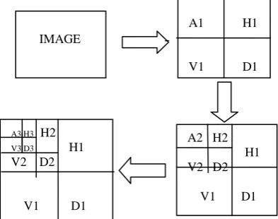
The discrete WT (DWT) is based on the fact that wavelet families are orthogonal or bi-orthogonal bases and do not produce redundant analysis. The DWT is computed by passing a signal successively through a high-pass and a low-pass filter. In the decomposition step, a signal is decomposed to a set of orthonormal wavelet function that constitutes a wavelet basis. The most common wavelets which provides the orthogonality properties are Daubechies, Symlets, Coiflets and Discrete Meyer. The result of the DWT is a multilevel decomposition in which the signal or image is decomposed in approximation and detail coefficients at each level. This is made through a process that is equivalent to low-pass and high-pass filtering, respectively. The decomposition sometimes called as the sub-band coding [4]. The image signal is considered as rows and columns as if they are one dimensional signal. In DWT, firstly the each row of the image is filtered, and then each of the columns is filtered. Figure 1 demonstrates the decomposition of an image for three levels. The result of this process gives four images: approximation (A), horizontal details (H), vertical details (V) and diagonal details (D). Because of sub-sampling after each filtering, the resultant sub-images have the quarter size of the original image. The proposed work uses Daubechies wavelet (db2) for the process of DWT. The db2 wavelets are a family of orthogonal wavelets characterized by a maximal number of vanishing moments.

Figure 1: DWT decomposition of an image for level 3.

2.3. Wavelet Thresholding

The wavelet coefficients which are the result of decomposition in wavelet transform is to suppress the small coefficients associated with the noise. After updating the coefficients by removing the small coefficients assuming as noise, the original signal can be obtained by the reconstruction algorithm using the noise free coefficients as it is considered that the noise has high frequency

In the linear penalization method every wavelet coefficient is affected by a linear shrinkage particular associated to the resolution level of the coefficient. The wavelet thresholding or shrinkage methods are usually more suitable. Donoho and Johnstone proposed a nonlinear strategy for thresholding where the threshold can be applied by implementing either hard or soft threshold method, which also called as shrinkage.

Hard and soft threshold with threshold λ are defined as follows:

The hard threshold operator is defined as

fh(x) = x if x ≥ λ = 0 otherwise The soft threshold operator is defined as

f (x) = x –λ if x ≥λ = 0 if x<λ

= x +λ if x ≤ λ

The advantage of this threshold appears in software implementation due to easy to remember and coding. The most known threshold selection algorithms are minimax, universal and rigorous sure threshold estimation techniques. The minimax method is used in statistics to design estimator. The minimax estimator realizes the minimum of the maximum mean square error, over a given set of functions.

The transfer function of the hard and soft threshold is shown in Figure 2.

(a) (b)

Figure 2: Threshold Types: a) Hard b) Soft

Another proposed threshold estimator method, introduced by Donoho [6], uses a threshold value T that is proportional to the standard deviation of the noise. It follows the hard thresholding rule. The threshold also referred to as universal threshold and it is defined as:

𝑇 = 𝜎 2 log 𝑀

Where, σ is the noise variance present in the signal and M represents the signal size or number of samples [2]. A threshold chosen based on Stein’s Unbiased Risk Estimator (SURE) [7] called as SureShrink, also known as A2 H2

H1 V2 D2

V1 D1 A3 H3 H2

V3 D3 H1 V2 D2

V1 D1 IMAGE

A1 H1

Where, t denotes the value that minimizes Stein’s Unbiased Risk Estimator, σ is the noise variance, and M is the size of the image.

3. SYSTEM MODEL

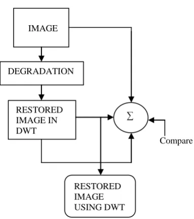
The proposed algorithm is depicted in the diagram (Figure 3). Let us consider an image of a particular size. The source image is corrupted by the various noise models:

 Gaussian noise.  Poisson noise  Salt and pepper noise  Speckle noise

Each noisy image degraded by the individual noise models is fed into the DWT.

Compare

Figure 3: Proposed Algorithm

The image is de-noised through the conventional process of DWT and the MSE is being calculated. At the receiver end, the aim is to remove the noisy components of the image such that the mean squared error is minimized through a dynamic process of the DWT. The calculated MSE is compared to a specified value till it is reduced to a certain extent and the process is made dynamic.

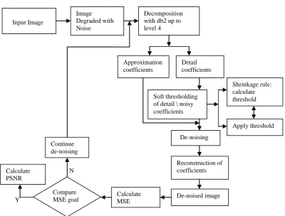
The flow diagram of the proposed dynamic DWT is described in the diagram (Figure 4).The related steps are: A clean image is considered as the source image. The image is then degraded by using the various noise types with varying variances. The degraded noisy image is fed for decomposition by the WT which is decomposed into sub-bands by wavelet packet transform using the orthogonal wavelet db2. The wavelet packet decomposes the degraded image into approximation and detail coefficients. The coefficients are extracted using the scaling and mother wavelet function.

The filtering process to decompose the image into coefficients is done by the wave filters constructed by the wavelet packet. The sub-band coding is done up to level 4 where for each level the approximation, diagonal, horizontal, and vertical coefficients forming the tree mode of the wavelet transform. The decomposed structure of the image is then thresholded by non-linear thresholding process in which only the detail coefficients are thresholded to eliminate the small coefficients of noise. The approximation coefficients are not thresholded. The soft thresholding technique is used to threshold the coefficients. The threshold is calculated using the Visu Shrinkage method expressed as,

𝑇 = 2 log 𝑛 ∗ 𝑠

Where, T is the threshold, n represents the product of the size of the noisy image and s is the estimation of the noise level.

The decomposed structure is then reconstructed using the reconstruction filter of the wavelet packet from level 4 to obtain the original de-noised image. The MSE is calculated for the noisy and de-noised image. The calculated MSE is checked with the MSE goal to minimize the error to a certain extent. If the MSE goal is reached the PSNR is calculated or else the de-noising process continues till the MSE goal is achieved (Figure 4). The data sets considered include several facial, scenic and medical images. Two sets are formed. One noise free used for referencing and the other corrupted by Gaussian, Salt and Pepper, Speckle and Poisson with variances from 0.02 to 0.09. The PSNR values of clean and restored images serve as the basis of performing the experiment.

4. EXPERIMENTAL DETAILS

The experiment is carried out by considering a gray scale image. The clean image is degraded by the individual noise models of varying variance/density from 0.02 to 0.09. The image is de-noised through the wavelet thresholding as mentioned in Section 3. The adaptive system model is use to perform the de-noising of the degraded image dynamically. The wavelet thresholding continues to de-noise the image till the MSE reduces to a constant value as specified. Here the constant value for the MSE is specified as 0.04. The image is decomposed up to level 4 by the wavelet. The decomposition level influences the frequency bands by dividing the sampling frequency.

IMAGE

DEGRADATION

RESTORED IMAGE IN DWT

∑

N

Y

Figure 4: Flow Diagram of dynamic DWT approach

If the higher decomposition level is used, the thresholding can eliminate some coefficients of the original signal, as in 1D signal de-noising process.

As shown in Table 1, the PSNR obtained for image degraded by additive Gaussian noise, the values of PSNR is almost constant and the values start decreasing after level 4 decomposition. Hence, the wavelet thresholding is done up to level 4. The wavelet thresholding uses the db2 wavelet to reconstruct the image up from the decomposed structure of the image. In the dynamic DWT process, the error is continuously compared to the MSE threshold to obtain the de-noise image. In this form it becomes visually more suitable than it was before the initiation of the process.

Table 1: PSNR values respect to decomposition level.

Level MSE PSNR

1 0.0723 59.28

2 0.0601 60.37

3 0.0554 60.73

4 0.0649 60.04

5 0.0705 59.68

6 0.0727 59.55

7 0.0730 59.53

8 0.0735 59.50

9 0.0730 59.53

10 0.0735 59.50

5. RESULTS AND DISCUSSION

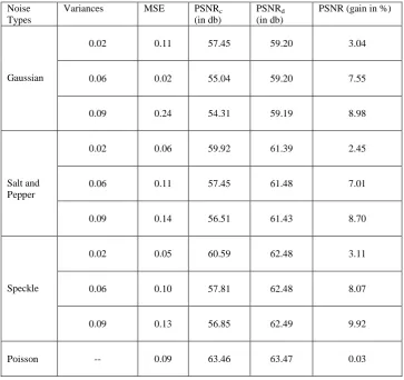
A set of experiments are performed using the MRI images of brain. The objective is to explore whether the proposed method is suitable for such applications. Initially an image corrupted by an individual noise model of variance 0.02 is considered. Next identical images corrupted by different other noises are used. The de-noised images obtained using both conventional and the proposed DWT based approaches are shown in Figures 5c and 5d respectively. Another set of results obtained are shown in Figures 6c and 6d. The PSNR values obtained by considering variances from 0.02 to 0.09 for respective noise models using dynamic DWT is shown in Table 2, where the PSNR values obtained through conventional process (PSNRc) and through proposed approach (PSNRd) is calculated. The PSNR values shows that there is an increase of 3.04 to 8.98% for Gaussian noise, 2.45 to 8.70% for Salt and Pepper noise, and 3.11 to 9.92% for Speckle noise in comparison to the values of PSNRc for the different noise types. However, the proposed process shows a subsequent increase of 3.04 to 9.92% in PSNR values in comparison to the conventional process. Table 3 shows the PSNR values obtained by using conventional DWT process for various variances values as done in [1]. Compared to the PSNR values reported in [1], the proposed dynamic WT approach shows a consistent improvement of around 46% which is significant. The Input Image

Image Degraded with Noise

Decomposition with db2 up to level 4

Approximation coefficients

Detail coefficients

Soft thresholding of detail \ noisy coefficients

De-noising

Reconstruction of coefficients

De-noised image

Shrinkage rule: calculate threshold

Apply threshold

Calculate MSE Compare

MSE goal Calculate

PSNR

Figure 5: a) Original image b) Gaussian Noise image of variance 0.02 c) De-noised image d) De-noised image of

dynamic WT

Figure 6: a) Original image b) Salt and Pepper Noise image of variance 0.09 c) De-noised image d) De-noised

image of dynamic WT

Table 2: PSNR values obtained for the varying values of variances 0.02 to 0.09 where PSNRc are the values obtained with conventional DWT, PSNRd are the values obtained with the proposed dynamic DWT and PSNR represents the gain

in % from conventional to the proposed dynamic process.

Noise Types

Variances MSE PSNRc

(in db)

PSNRd (in db)

PSNR (gain in %)

Gaussian

0.02 0.11 57.45 59.20 3.04

0.06 0.02 55.04 59.20 7.55

0.09 0.24 54.31 59.19 8.98

Salt and Pepper

0.02 0.06 59.92 61.39 2.45

0.06 0.11 57.45 61.48 7.01

0.09 0.14 56.51 61.43 8.70

Speckle

0.02 0.05 60.59 62.48 3.11

0.06 0.10 57.81 62.48 8.07

0.09 0.13 56.85 62.49 9.92

Table 3: PSNR for conventional DWT based approach for Gaussian noise

Variances MSE PSNR (in db)

20 0.44 51.72

30 0.445 51.68

40 0.447 51.65

50 0.4490 51.65

6. CONCLUSION

Here we proposed a dynamic WT based de-noising approach for images corrupted by Gaussian noise. The proposed approach provides 2.45 to 9.92% improvement in PSNR values. Also the proposed method provides up to 46% improvement in PSNR values of de-noised images compared to [1]. Thus, the proposed approach can be part of image processing application requiring appropriate restoration quality for biomedical imaging system as it offers higher PSNR values in comparison to [8] and [9].

7. REFERENCES

[1] P.Hedaoo and S.S.Godbole, ʻʻWavelet Thresholding Approach for Image Denosing”, International Journal of Network Security & Its Applications (IJNSA), vol.3, no.4, pp. 16-21, 2011.

[2] H.Om and M.Biswas, ʻʻAn Improved Image Denoisng Method Based On Wavelet Thresholding”, Journal of Signal and Information Processing, vol 3, pp.109-116, 2012.

[3] R. K. Rai and T. R. Soutakke, ʻʻImplementation of Image Denoising Using Thresholding Techniques”, International Journal of Computer Technology and Electronics Engineering (IJCTEE) vol 1, issue 2, pp.6-10.

[4] A.Bijalwan, A.Goyal and N.SethI, ʻʻWavelet Transform Based Image Denoise Using Threshold Approaches”, International Journal of Engineering and Advanced Technology (IJEAT), vol. 1, issue-5, pp.6-10, 2012. [5] S.G. Chang and M. Vetterli, “Adaptive Wavelet

Thresholding For Image Denoisng And Compression”, IEEE Transactions On Image Processing, vol. 9, no. 9, pp. 1532 1546, 2000.

[6] D.L.Donoho, ʻʻDenoising by Soft Thresholding”, IEEE Transactions On Information Theory, vol. 41, no. 3, pp.613-627, 1995.

[7] X. Zhang, ʻʻAdaptive Denoising Based On Sure Risk”, IEEE Signal Processing Letters, vol. 5, no. 10, pp.2-8, 1998.

[8] S.Khan, A.Jain and A.Khare, “Image denoising based on adaptive wavelet thresholding by using various shrinkage methods under different noise condition”, International Journal of Computer Applications, vol.59, no.20, pp. 13-17, 2012.