Simplex Optimization and Its Applicability for Solving Analytical Problems

http://dx.doi.org/10.4236/jamp.2014.27080

How to cite this paper: Michałowska-Kaczmarczyk, A.M. and Michałowski, T. (2014) Simplex Optimization and Its Applica- bility for Solving Analytical Problems. Journal of Applied Mathematics and Physics, 2, 723-736.

http://dx.doi.org/10.4236/jamp.2014.27080

Simplex Optimization and Its Applicability

for Solving Analytical Problems

Anna Maria Michałowska-Kaczmarczyk1_{, Tadeusz Michałowski}2* 1_{Department of Oncology, The University Hospital in Cracow, Cracow, Poland}

2_{Faculty of Engineering and Chemical Technology, Cracow University of Technology, Cracow, Poland}

Email: *_{[email protected]}

Received 14 April 2014; revised 14 May 2014; accepted 21 May 2014

Copyright © 2014 by authors and Scientific Research Publishing Inc.

This work is licensed under the Creative Commons Attribution International License (CC BY).

http://creativecommons.org/licenses/by/4.0/

Abstract

Formulation of the simplex matrix referred to n-D space, is presented in terms of the scalar prod- uct of vectors, known from elementary algebra. The principles of a simplex optimization proce- dure are presented on a simple example, with use of a target function taken as a criterion of opti- mization, where accuracy and precision are treated equally in searching optimal conditions of a gravimetric analysis.

Keywords

Simplex, Simplex Optimization Procedure

1. Introduction

Simplex is a geometric figure, formed on the basis of n+1 points A i_i

(

=0,,n

)

in the n-dimensional space, i.e., a number of the points exceeds the dimension of the space by one. These points are referred to as the vertic- es of the simplex. Distribution of the points Ai in this space is represented by a matrix of this simplex. Speci-

fying the coordinates for Ai is easy if it concerns the 2-D or 3-D space, but it becomes less comprehensi-

ble when the issue concerns the n-dimensional

(

n D-

)

simplex. Although in the literature [1] one can find ready-made forms of the simplex matrix in n D- space, but information on how to receive it in an easy manner is lacking.

is widely applicable and popular in different fields of chemistry, chemical engineering, and medicine [9]. Fur- thermore, it works well in practice on a wide variety of problems, where real-valued minimization functions with scalar variables are applied.

The sequential simplex method is considered as one of the most effective and robust methods applied in me- thodology of Evolutionary Operation (EVOP) experimental design [10]-[15]. The SOP method was implement- ed in MINUIT (a Fortran from CERN [16] package), then in Pascal, Modula-2, Visual Basic, and C+ + [17]. The iterations are stopped when the function minimized is less than a preset value.

In this article, the problem of obtaining the simplex matrix in n D- space will be presented on the basis of the triangle and the scalar product concept, well-known to the students from earlier stages of education. The evolution of the simplex according to SOP [3] [18] will also be presented in a understandable manner.

2. Simplexes in 2-

D

and 3-

D

Space

In order to introduce the simplex concept, we start from the point

(

0-D

)

, (I) segment

(

1-D

)

, (II) equilateral triangle

(

2-D

)

, and (III) tetrahedron

(

3-D

)

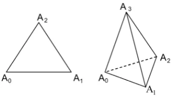
concepts, known from the elementary geometry. The 0-D, 1-D, 2-D, 3-D (and generally n D- ) notations express the dimensionality of the corresponding geometrical enti- ties (Figure 1).

The points: A0, A1, A2 are vertices of the triangle A A A0 1 2; the points: A0, A1, A2, A3 are the vertices of the tetrahedron A A A A0 1 2 3. A A0 1 is one of the edges of the triangle; A A0 1 is one of the edges of the tetrahe- dron. Equilateral triangle A A A0 1 2 is one of walls of the tetrahedron.

Segment, equilateral triangle, and tetrahedron can be presented in the same scale; it means that all distances, equal to unity (chosen arbitrarily), between the (neighbouring) points Ai and Aj of a polygon are assumed, i.e.

the length A Ai j =1.

All angles between edges of the equilateral triangle are equal to 60˚

(

π 3rd

)

. All angles between adjacent tetrahedron edges are equal 60˚ too, owing to the fact that all the tetrahedron walls are composed of equilateral triangles

(

2-D

)

. By turns, tetrahedrons form the 3-D walls in 4-D polygon, etc. It means that all angles between adjacent edges of a symmetrical n D- polygon are equal 60˚, as well.

The equilateral triangle can assume different positions on the plane. A particular case is the triangle with unit edges, “anchored” at the origin of co-ordinate axis, as one presented in Figure 2.

The successive vertices of the equilateral triangle can be presented in matrix form, where the rows are ex- pressed by co-ordinates of the corresponding points A i_i

(

=0,1, 2

)

:

0

1

2

0 0

1 0

1 2 3 2 A A A

 

 

=  

 

 

X (1)

The second and third rows of this matrix are identical with components of transposed vectors: A A0 1 and 0 2

A A , respectively:

[ ]

T

[

]

T

0 1 1, 0 , 0 2 1 2 , 2

A A = A A =

The tetrahedron can assume different positions in 3-D space. A particular case is the tetrahedron anchored at the origin of co-ordinate axis as one presented in Figure 3.

The successive vertices of the tetrahedron can be presented in the matrix form:

0

1

2

3

0 0

0

0 0

1

0 1 2 3 2 1 2 3 6 6 3

A A A A

 

 

 

=  

 

 

 

X (2)

The second, third and fourth rows of this matrix are identical with components of the transposed vectors:

0 1

A A , A A0 2 and A A0 3, respectively:

[

]

_T T T

[image:3.595.227.398.83.181.2]

Figure 1. Equilateral triangle and tetrahedron.

Figure 2. The equilateral triangle with unit edges and points: A0

( )

0,0 ; A1

( )

1,0 ; A2

(

0.5, 3 2

)

.

Figure 3. The tetrahedron with unit edges and

(

)

0 0,0,0

A ; A1

(

1,0,0

)

; A2

(

1 2, 3 2,0

)

;

(

)

3 1 2, 3 6, 6 3

A .

3. Simplexes in

n

-

D

Space

The segment, equilateral triangle and tetrahedron are imaginable concepts. However, application of the concepts involved with geometric figures of higher dimension

(

n≥4

)

is beyond imagination. One should be taken into account that, in the simplex optimization, we are forced, as a rule, to consider higher number of factors influ- encing the optimizing process.

[image:4.595.163.429.534.699.2]

Figure 4. Formation of consecutive dimensions (up to 5-D) of a simplex in projective space.

Let us assume that the polygon is “anchored” in n-D-space in such a manner that A0 is in the origin of the co-ordinate axis and any successive point “enters” the new dimension of the n-D-space, see Figure 4. It means that the co-ordinates of the corresponding points of n D- polygon are as follows:

(

)

(

)

(

)

(

)

(

)

(

)

0 1 11 2 21 22 3 31 32 33

1 1,1 1,2 1,3 1, 1 1 2 3 , 1

0, 0, 0, , 0, 0 ; , 0, 0, , 0, 0 ; , , 0, , 0, 0 ; , , , , 0, 0 ; ;

, , , , , 0 ; , , , , , .

n n n n n n n n n n n n nn

A A x A x x A x x x

A− x− x− x− x− − A x x x x − x

= = = =

= =

    

  (3)

This means that xij =0 for j>i.

As stated above, the number of vertices exceeds, by 1, the dimension of the space; it means that the polygon in

-n D space involves n+1 vertices.

We consider a pencil of n unit vectors, xi= A A0 i=

[

xi1,xi2,xi3,,xii,,xin

]

T, all starting from the point

(

)

0 0, , 0

A =  , i.e., origin of co-ordinates of n D- space and ending at the points A i_i

(

=1, 2,,n

)

. One should notice that the basic components xij of the vector xi starting at the origin of co-ordinates, are

identical with co-ordinates of the point Ai =

(

xi1,xi2,xi3,,xij,,xin

)

. Then for the vectors A A0 i based on the

points specified in (3) we have:

[

]

[

]

[

]

[

]

[

]

T 1 0 1 11

T 2 0 2 21 22

T 3 0 3 31 32 33

T

0 1 2 3

T

0 1 2 3

, 0, 0, , 0 ;

, , 0, , 0 ;

, , , 0, , 0 ;

, , , , , 0, , 0 ;

, , , , , , .

i i i i i ii

n n n n n ni nn

A A x A A x x A A x x x A A x x x x

A A x x x x x

= = = = = = = = = =        x x x x x (4)

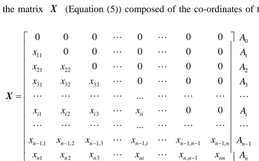
Let us construct the matrix X (Equation (5)) composed of the co-ordinates of the corresponding points in

-n D space:

0

11 1

21 22 2

31 32 33 3

1 2 3

1,1 1,2 1,3 1, 1, 1 1, 1

1 2 3 , 1

0 0 0 0 0 0

0 0 0 0 0

0 0 0 0

0 0 0

...

0 0

...

i i i ii i

n n n n i n n n n n

n n n ni n n nn n

A

x A

x x A

x x x A

x x x x A

x x x x x x A

x x x x x x A

− − − − − − − − −               =                                            

X (5)

trix X =   xij can be specified as follows:

(

)

(

)

0 for

0 for , 1,

0 for 0 1, ,

ij

i j

x i j i j n

i j n

> ≥

 

= < ∈< >

 _{= =}

 

(6)

Let ei be the unit vector along the i-th axis, Xi, i.e. ei =1. The ej vectors form a set of mutually orthogo-

nal vectors in n-D space. The scalar products:

(

)

1 for

cos ,

0 for

i j i j i j ij

j i j i

δ  =

⋅ = ⋅ ⋅ ∠ = _{= }

≠ 

e e e e e e (7)

where δij is the Kronecker symbol.

Any vector xi in n D- space can be also written as

[

]

T 1 2

x , x , , x

i= i i  in

x ; 1 k

n i =

∑

k= ⋅xik

x e . Then the

scalar product of two vectors, xi and xj, in n D- space is as follows:

(

)

1

cos , n

i⋅ j = i ⋅ j ⋅ ∠ i j =

∑

k= x xik jk

x x x x x x (8)

where ∠x xi, j is the angle between vectors xi and xj spanning the simplex in n D- space. The angle be-

tween different vectors xi =A A0 i and xj= A A0 j of n D- simplex equals π 3 [rd], i.e.

o

, 60

i j

∠x x =

and then

(

)

o

cos ∠x xi, j =cos60 =1 2, for any pair of the vectors xi and xj: in triangle

(

2-D

)

, in tetrahe-

dron

(

3-D

)

,. Moreover, ∠x xi, i =0 and then cos

(

∠x xi, j

)

=cos0=1. If the unit vectors xi

(

i=1,,n

)

are assumed, i.e., xi =xi =1, then from (8) and (4)-(6) we have:

( )

1 1

1

where min , 2

n m

ik jk ik jk

k= x x = k= x x = m= i j

∑

∑

(9)

2

1 1, where 1, ,

i ij

j= x = i= n

∑

 (10)

From (9), (10) and (6) we get, by turns,

1 2 2

11 11 1

1 1 1 1

2 1 x = → x = =_ + _ =h

⋅

 

11 1 2

1

0 0 0 0 0 0

2

i i ii

x ⋅x + ⋅x + + ⋅ x + ⋅ + + ⋅ = , i.e.

(

)

11 1 1 1

1 1

1 2 for 2, ,

2 1 1

i i

x ⋅x = i= n → x = = ⋅h

+



(

for 2≤ ≤i n

)

(

)

1 2 2 1 2 1 2

2 2 2

21 22 22 21 2

1 3 2 1

1 1 1

2 2 2 2

x +x = → x = −x = −_ _{ }  _ = =_ + _ =h

⋅

   

 

21 1 22 2 2 2

1 1 3 1

?

2 3 2 2 1

i i i

x ⋅x + x ⋅x = → x = = h

+

(

for 3≤ ≤i n

)

(

)

1 2

1 2

2 2 2 2 2

31 32 33 33 31 32 3

6 3 1

1 1

3 2 3

x +x +x = → x = −x −x = =_ + _ =h ⋅

 

31 1 32 2 33 3 3 3

1 1 6 1

2 4 3 3 1

i i i i

x ⋅x + x ⋅x + x ⋅x = → x = = h

+

(

for 4≤ ≤i n

)

(

)

1 2

1 2

2 2 2 2 2 2 2

41 42 43 44 44 41 42 43 4

10 4 1

1 1

4 2 4

x +x +x +x = → x = −x −x − x = =_ + _ =h ⋅

41 1 42 2 43 3 44 4 4 4

1 1 10 1

2 5 4 4 1

i i i i i

x x +x x +x x +x x = → x = = h

+

(

for 5≤ ≤i n

)

and so forth. On this basis, one can write:

(

)

1 2 1 for 1 2 jj j j

x h j n

j

 + 

= =_{ } ≤ ≤

  (11)

(

)

(

)

1 2 1 2

1 1 1

for

1 2 2 1

ij j

j

x r j i n

j j j j

 

 + 

= = ₊   =_{ +} _ < ≤

    (12)

The elements xij of the matrix X=   xij (Equation (5)) are thus derived with use of principles of elemen-

tary algebra and geometry. Then the n D- simplex can be written in the form

1

1 2

1 2 3

1 2 3

0 0 0 0

0 0 0

0 0

0

n

h r h r r h

r r r h

        =             X           (13)

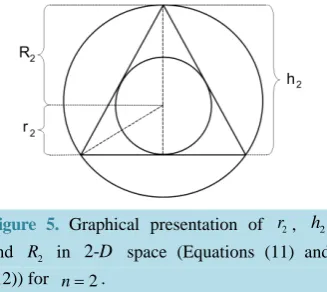
One can notice that hj (Equation (15)) is the height of j D- symmetrical simplex and rj (Equation (16)) is

the radius of -j D sphere (for j=2—circle, for j=3—“normal” sphere) inscribed in -j D simplex. Moreover, we have the relations:

and

j j j j j

h = +r R R = ⋅j r (14)

where Rj is the radius of j D- sphere circumscribed on j D- simplex, see Figure 5.

In particular, for n=7, the matrix X (Equation (13)) has 7 columns and 8 rows.

0 1 2 3 4 5 6 7

0 0 0 0 0 0 0

1 0 0 0 0 0 0

0.5 0.866 0 0 0 0 0

0.5 0.289 0.817 0 0 0 0

0.5 0.289 0.204 0.791 0 0 0

0.5 0.289 0.204 0.158 0.775 0 0

0.5 0.289 0.204 0.158 0.129 0.764 0

0.5 0.289 0.204 0.158 0.129 0.109 0.756 A A A A A A A A             =              

X (15)

4. Translation and Reflection of the Simplex

A simplex can be translated and/or rotated in space. Particularly, the simplex defined by X (Equation (13)), with the centre at Ac =

(

r1,,rn

)

, can be parallely shifted to the centre Pc0=

(

0,, 0

)

of the co-ordinate sys-

tem. This way, one obtains a new matrix Xtr

1 2 3 1

1 2 3 1

2 3 1

1 0

0 0 0

0 0 0 0

n n n n n n tr n n n

r r r r r

R r r r r

R r r r

Figure 5. Graphical presentation of r2, h2

and R₂ in 2-D space (Equations (11) and (12)) for n=2.

with Rj and rj

(

j=1,,n

)

as ones in Equations (11), (12) and (14). Reflection of particular vertices of the matrix Xtr in the centre of co-ordinate system

(

0,, 0

)

gives the simplex described by the matrix

( )

1 2 3 1

1 2 3 1

2 3 1

1 0

0 0 0

0 0 0 0

n n n n n n tr n n n

r r r r r

R r r r r

R r r r

R r R − − − ∗ −   ₋     −  = ⋅ − =      ₋    −    

X X I

           (17)

where I=   δij —identity matrix.

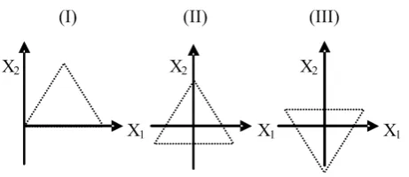
The positions of the simplex presented in Figure 6 (in 2-D space), obtained from (I) by translation (II) and mirror reflection (III) in the origin of ordinate axis, are presented by matrices: Xtr and:

∗

X (Equation (21) for 2

n= and

1 2

1 2

2

0.5 0.289

0.5 0.289

0 0 0.578

tr r r R r R − − − −         =_ − _{ }= − _         X 1 2 1 2 2 0.5 0.289 0.5 0.289

0 0 0.578

r r R r R ∗         = −_{  }= − _  −   −      X

Note that the number of k D- walls in n D- simplex equals to the number of k+1 point subsets (k D -walls) generated from the n+1-point set. From the elementary theory of combinations it results that the num- ber of k-D walls equals to the number of possible combinations of n+1 items taken k+1 at a time, i.e.

( )

1

₍

(

_{) (}

1 !

)

₎

,

1 1 ! !

n n

N n k

k k n k

+ +

 

=_{ }=

+ + −

  (18)

Particularly, 3-D simplex (tetrahedron, n=3) involves N

( )

3, 2 =4 triangles (2-D walls), N

( )

3,1 =6 edges (segments, 1-D walls) and N

( )

3, 0 =4 points (vertices, 0-D walls). Generally, the n D- simplex consists of: N n

( )

, 0 = +n 1 vertices of the virtual solid stretched on them, N n

( )

,1 =n n

(

+1 2

)

edges, ,

(

, 1

)

1

N n n− = +n of

(

n 1 -−

)

D walls opposite to particular vertices.

5. Simplex Optimization Procedure (SOP)

[image:7.595.233.397.83.229.2]

[image:8.595.199.430.82.182.2]

Figure 6. The simplexes obtained after successive (II) transla- tion and (III) reflection of the original simplex (I) in the center of co-ordinate axes in 2-D space; for details—see text.

securing optimal accuracy and precision of an analytical method.

5.1. An Objective Function

The simplex concept is applicable, among others, for optimisation of analytical methods [13]. The variables, xi

(scalars), named as factors forming the vector x, affect the variable y, named as objective (“target”) function, i.e.,

( )

(

1, , n

)

y= y x = y x  x (19)

The essence of optimisation is inherent in the objective function. Accuracy and precision are among the most important criteria of analytical methods. Another object functions are related to sensitivity of a method, effi- ciency of a chemical reaction, etc.

Let us assume that an analytical method aims to find the conditions securing true contents

(

m0, g g

)

of an

analyte in a sample to be obtained. For this purpose, the following criterion (objective function)

( )

(

) (

2

)

₂

2

0 0

1

1 1

1

i N

ik i i

k

i i

y i m m m m s

N = N

 

= − = − + −_{ }⋅

 

∑

(20)

has been suggested [19], where:

1 1 Ni

i k i k

i

m m

N =

= ⋅

∑

(21)

(

)

2 2

1 1

1

i N

i k ik i

i

s m m

N =

= ⋅ −

−

∑

(22)

were calculated in the i-th simplex point, Ai (Equation (3)), on the basis of Ni measurements mik of an

intensive variable m (e.g. number of grams of an analyte contained in a unit mass of solution); m0 is the true value of this variable, obtained according to a reference method. In the object function (20), both terms, i.e. ac- curacy

(

m– m0

)

and precision, expressed by standard deviation,

2

i i

s = s , are considered nearly equivalently; the difference in “weights”: 1 and 1 1− Ni , of the two characteristics of the method becomes less significant

at higher Ni values.

The function (20) is an example of superposition of different characteristics of a method, i.e. accuracy and precision. The optimisation is terminated when the systematic error is insignificant, i.e., the inequality

(

)

0 0.95,

i

i i

i s

m m t f

N

− < ⋅ (23)

is fulfilled; 0.95, t

(

f_i

)

is the critical t-value of the Student’s t-test at fi =Ni−1 degrees of freedom, on 95% probability level pre-assumed. In particular, for Ni =4, i.e. fi =3, we have t

(

0.95, 3

)

=3.182, and then Eq-

uation (23) has the form

i

i m s

5.2. Decision Variables and Arrangement of Experimental Conditions The optimization procedure assumes:

1) Selection of natural decision variables, Zi, as independent (in principle) individual factors affecting the

values of the objective function (Equation (19)) and 2) Their order, Z_j

(

j=1,,n

)

.

The number

( )

n of the variables Zj chosen defines the simplex dimension.

The kind

( )

Zj and the number

( )

n of these variables that assume continuous (not discrete) values

(

1, ,

)

j

z j=  n , consisting the vector z=

(

z1,,zn

)

T, affects the success (efficiency) of optimisation process

aiming to get optimal (maximal or minimal) value for the object function, e.g. minimal value for y=y i

( )

de- fined by Equation (20). It should be noted that the n D- simplex matrix (Equation (5)) refers—in principle—to orthogonal (independent) variables. The independent variables assuming continuous values are, among others: pH, temperature, time, rate of an operation.

One should be noticed that the form of the matrix (5) enables to add a new variable, Zn+1, to the set of n va- riables Z1,,Zn assumed at the start for optimization—provided that the decision of inclusion of variable

1

n

Z + into the set of variables has been undertaken after measurements done in the points A0,,Ap, at p≤n,

where Zn+1 remained unchanged. In this case, the measurements done at the points A0,,Ap has not to be

repeated.

5.3. Design of Experiments and Optimization within the Starting Simplex

The introductory step of the optimization procedure assumes fixing the starting values, z0j, and steps, ∆zj,

assumed for Z_j

(

j=1,,n

)

; these values affect strongly the efficiency of the optimization procedure. Some constraints put on zj and ∆zj values (resulting from physicochemical, chemical or technological reasons)

can also be taken into account. These constraints may result e.g., from limited solubility, possibility of phase change affected by temperature, etc.

The optimization is realized there for values of natural variables calculated from the formula

0

ij j ij j

z =z + ⋅ ∆x z (25)

where i=0,1,,n enumerates successive experimental points realized within the initial simplex. The advised values for xij in (5) are defined in the matrix (13) and specified e.g. in the matrix (15) if n=7. The values

( )

, 0, ,

y j j=  n, obtained at n+1 points A A0, 1,,An of the initial simplex are the basis for its further

evolution of the simplex.

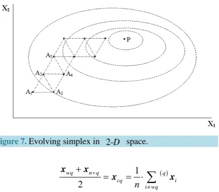
5.4. Optimization at the Points of Evolving Simplex

At the first stage of the simplex evolution (Figure 7), a point Aw1 with the worst

( )

w1 value, y w

( )

1 , for the object function (Equation (20)) is indicated, w1∈<0,n>. The point Aw1 is replaced by a new point,

1

n

A+ , obtained by reflection of Aw1 in the centre, Ac1

( )

xc1 , of the remaining n points of the initial simplex,

i.e., in n−1-D wall not containing the point Aw1. In other words, xc1 is the middle point between xw1 and n 1+

x , i.e.,

1 1

1

1 1 2

w n

c i

i w

n

+

≠

+ _{= = ⋅}

∑

x x

x x (26)

After adding the term

( )

1n ⋅x_w1 to both sides of Equation (26), we obtain the co-ordinates of the new point, 1

n

A+ ,

1 1

1

2 2

1

n

n i w

i

n n

+ =

 

= ⋅ − +_{ }⋅

 

∑

x x x (27)

[image:10.595.202.427.85.282.2]

Figure 7. Evolving simplex in 2-D space.

( ) 1 2

wq n q q

cq i

i wq

n

+

≠

+

= = ⋅

∑

x x

x x (28)

In the example presented above, the initial (symmetrical) shape of the evolving simplex is maintained owing to the fact that 1) mirror reflections are applied and 2) equal statistical weights are assumed to all the simplex points considered. Sometimes we are forced to move the simplex within a constrained component space [20].

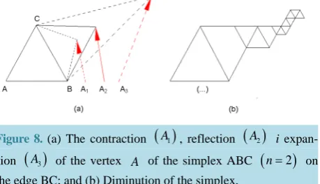
The evolving simplex approaches the quasi-optimal region, where y i

( )

values do not change distinctly. In this region, the evolving simplex should be contracted or diminished (Figure 8); such operations enter e.g. the MINUIT program. The contraction/dilatation and weighting are involved in the relation [21] [22]

(

1

)

n q+ = −α ⋅ wq+ ⋅α cq

x x x (29)

where the parameter α results from re-parametrization of the a line passing through 2 points: one of them is xwq,

the second one is the centre xcq of area of q-th, n 1-D− simplex, defined as follows

( )

( ) q

i i i wq

cq q

i i wq

p

p ≠

≠

=

∑

∑

x

x (30)

where the operator ( )q i wq

∑

≠

means summation within q-th n 1-D− simplex (xwq excluded). The contraction or

expansion and weighting (“weights” pi) different points xi deforms the evolving simplex gradually. As a rule,

it is not an advantageous occurrence during the optimization procedure, however. The simplex deformation is influenced mainly by the weighting factors [23]. Moreover, a shape of response function may sometimes cause the optimum searching impossible, even in 2-D space.

6. Example of SOP

To illustrate the principle of SOP, a simple example of gravimetric analysis is considered below. The matrix ex- pressed by Equation (15) was chosen for initial simplex, and Equation (20) was applied as criterion of optimiza- tion. Ni=4 measurements were made at each simplex point. In our case, the relation (24) is chosen as the cri- terion of optimization. Analyses were made with CdSO4 solution of

(

m0=0.01272 gCd / 1g

)

, standardised ac-

cording to electrogravimetry, considered as the reference method.

6.1. Analytical Prescription

Figure 8. (a) The contraction

( )

A1 , reflection

( )

A2 i expan-

sion

( )

A3 of the vertex A of the simplex ABC

(

n=2

)

on

the edge BC; and (b) Diminution of the simplex.

6.2. Decision Variables

Z1—re-crystallisation time [min] of the precipitated CdL2; Z2—mass [g] of tartaric acid added in the solution;

Z3—volume [ml] of NaOH added;

Z4—volume [ml] of 8-hydroxyquinoline added; Z5—rate [ml/min] of 8-hydroxyquinoline addition;

Z6—temperature [˚C] of water bath where re-crystallization of CdL2 occurs; Z7—volume [ml] of the solution before precipitation.

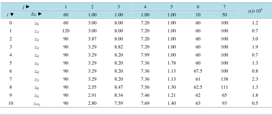
For example, the value z04=7.20 [ml] refers to variable Z4; the related value ∆ =z4 1.00 ml. For i=3 and 4

j= , from Table 1 we have z34=8.00+0.817 1.00× ≅8.82.

6.3. Results of Analyses within the Initial Simplex

The simplex optimisation procedure was realized in experiments performed in all points of the initial simplex (rows 0,, 7 in Table 1). In each point A i_i

(

=0,, 7

)

, Ni=4 measurements were done. The results mik[gCD/g] are presented in Table 2.

On the basis of the data in Table 2, the y i

( )

values were calculated (last column in Table 1).

As results from detailed calculations done on the basis of results in Table 2, the inequality (23) has not been fulfilled within the initial simplex and then the evolution of the simplex was needed.

Referring to theTable 1, the worst

(

w=w1

)

result within the initial simplex was obtained at the point A2. During the simplex evolution, this point was reflected in the centre xc1 of the remaining points of the starting simplex. Referring toTable 1, we have, for example,

(

)

2 1c 2 0 5 0.289 7 0.206

x = ⋅ + × =

(

0.866+x82

)

2=0.206 → x82 = −0.454

(

)

82 3.00 0.454 1 2.55

z = + − × ≅

(

)

3 1c 2 0 0.817 4 0.204 7 0.233

x = × + + × =

(

0+x83

)

2=0.233 0.466→ x83 =

83 8.00 0.466 1 8.47

z = + × ≅

At the point A8, the condition (24) has not been fulfilled as well, and further evolution of the simplex was required. The worst y w

( )

2 value within the new simplex was stated in the point A7. Further calculations re- ferred to the new point A9 are exemplified below:

(

)

(

)

2 2c 2 0 4 0.289 1 0.454 7 0.1004

x = × + × + × − =

(

0.289+x92

)

2=0.1004 → x92= −0.088,

(

)

92 3.00 0.088 1 2.91

[image:11.595.200.430.92.224.2]

[image:12.595.87.538.114.304.2]

Table 1. The values for zij assumed in points of the initial (columns 1-7, rows 0-7) and evolving (columns 1-7, rows 8-10)

simplexes. For all points, the values y i

( )

were obtained on the basis of N_i=4 measurements.

j► 1 2 3 4 5 6 7

y(i)⋅108

i ▼ ∆zi ► 60 1.00 1.00 1.00 1.00 10 50

0 z0j 60 3.00 8.00 7.20 1.00 60 100 1.2

1 z1j 120 3.00 8.00 7.20 1.00 60 100 0.7

2 z2j 90 3.87 8.00 7.20 1.00 60 100 3.0

3 z3j 90 3.29 8.82 7.20 1.00 60 100 1.9

4 z4j 90 3.29 8.20 7.99 1.00 60 100 0.7

5 z5j 90 3.29 8.20 7.36 1.78 60 100 1.3

6 z6j 90 3.29 8.20 7.36 1.13 67.5 100 0.8

7 z7j 90 3.29 8.20 7.36 1.13 61 138 2.3

8 z8j 90 2.55 8.47 7.56 1.30 62.5 111 1.3

9 z9j 90 2.91 8.34 7.46 1.21 62 65 1.8

10 z10,j 90 2.80 7.59 7.69 1.40 63 93 0.5

Table 2. Results of measurements done within the initial simplex.

A0 A1 A2 A3 A4 A5 A6 A7

0.01260 0.01263 0.01257 0.01268

0.01265 0.01268 0.01259 0.01265

0.01256 0.01252 0.01249 0.01267

0.01256 0.01258 0.01269 0.01255

0.01265 0.01267 0.01260 0.01264

0.01262 0.01255 0.01267 0.01262

0.01262 0.01268 0.01261 0.01264

0.01255 0.01259 0.01262 0.01253

(

)

3 2c 2 0 0.817 3 0.204 0.467 7 0.271

x = × + + × + =

(

0.204+x93

)

2=0.271 0.338→ x93=

93 8.00 0.338 1 8.34

z = + × ≅

(

)

7 2c 6 0 0.216 7 0.031

x = × + =

(

0.756+x97

)

2=0.031 → x97 = −0.694,

(

)

97 100 0.694 50 65

z = + − × ≅ .

The coordinates of the new points: A8, A9 and A10 for evolving simplexes, calculated with use of the coded variables xij specified.

8 9 10

0.5 0.454 0.467 0.361 0.295 0.249 0.216

0.5 0.088 0.338 0.261 0.214 0.180 0.694

0.5 0.196 0.412 0.494 0.404 0.341 0.137 A

A

A

−

 

 _{− −} 

 

 − − − 

 

The optimisation procedure has been terminated at the point A10, where mi =0.01267 and variance

2 8

0.32 10 i

s = × − were found on the basis of 4 measurements and then the inequality (24)

4 4

0.01267 0.01272− <0.56 10× − ×1.591=0.89 10× −

was fulfilled and

( ) (

) (

2

)

8 8 8

10 0.01267 0.01272 1 1 4 0.32 10 0.49 10 0.5 10

y = − + − × × − = × − ≅ × −

6.4. Optimal Prescription

On the basis of the optimization procedure, one can formulate the following prescription.

[image:12.595.90.539.318.377.2]

taken for analysis. The solution was treated with 2.80 g of tartaric acid and then with 7.9 ml of 2.5 mol/l NaOH solution. After dilution with water up to ca 90 ml, the solution was treated with 7.7 ml of 3% (m/v) 8-hydroxy- quinoline solution (added dropwise from burette, with the rate 1.4 ml/min. The mixture was leaved for ca. 90 min on the water-bath for re-crystallisation of the precipitate CdL2 at temperature 63˚C, then filtered, washed with water, dried to a constant mass at 105˚C and weighed.

7. Final Comments

In this paper, the simplex method has been presented in terms known from elementary algebra and geometry. On the basis of scalar product and length of vectors in normalized scale, the co-ordinates of simplex vertices in

-n D space were determined. A criterion of optimization, where accuracy and precision of measurements were considered equivalently, has been suggested.

The simplex method was considered as the most efficient among optimization procedures, applicable in si- mulating procedures realized in recursive computer programs used for simulation purposes and in optimization of analytical procedures. The simplex method requires only one additional experiment, regardless of the number of factors being varied. This drastically reduces the number of experiments required to reach the optimum.

References

[1] Anderson, V.L. and McLean, R.A. (1974) Design of Experiments: A Realistic Approach. Marcel Dekker, Inc., New York, 363.

[2] Nelder, J.A. and Mead, R. (1965) A Simplex Method for Function Minimization. Computer Journal, 7, 308-313.

http://dx.doi.org/10.1093/comjnl/7.4.308

[3] Walters, F.H., Parker, L.R., Morgan, S.L. and Deming, S.N. (1991) Sequential Simplex Optimization. CRC Press, Bo- ca Raton. http://www.chem.sc.edu/faculty/morgan/pubs/SequentialSimplexOptimization.pdf

[4] Spendley, W., Hext, G.R. and Himsworth, F.R. (1962) Sequential Application of Simplex Designs in Optimisation and Evolutionary Operation. Technometrics, 4, 441-461. http://dx.doi.org/10.1080/00401706.1962.10490033

[5] Fletcher, R. (1965) Function Minimization without Evaluating Derivatives—A Review. Computer Journal, 8, 33-41.

http://dx.doi.org/10.1093/comjnl/8.1.33 http://folk.uib.no/ssu029/Pdf_file/Fletcher65.pdf

[6] Olsson, D.M. and Nelson, L.S. (1975) The Nelder-Mead Simplex Procedure for Function Minimization. Technome- trics, 17, 45-51. http://dx.doi.org/10.1080/00401706.1975.10489269

[7] Fletcher, R. and Powell, M.J.D. (1963) A Rapidly Convergent Descent Method for Minimization. Computer Journal, 6, 163-168. http://dx.doi.org/10.1093/comjnl/6.2.163

[8] Fletcher, R. and Reeves, C.M. (1964) Function Minimization by Conjugate Gradients. Computer Journal, 7, 149-154.

http://dx.doi.org/10.1093/comjnl/7.2.149

[9] Lagarias, J.C., Reeds, J.A., Wright, M.H. and Wright, P.E. (1998) Convergence Properties of the Nelder-Mead Simp- lex Algorithm in Low Dimensions. SIAM Journal of Optimization, 9, 112-147.

http://dx.doi.org/10.1137/S1052623496303470

http://citeseerx.ist.psu.edu/viewdoc/download?doi=10.1.1.120.6062&rep=rep1&type=pdf

[10] Box, G.E.P. and Hunter, J.S. (1957) Multi-Factor Experimental Designs for Exploring Response Surfaces. Annals of Mathematical Statistics, 28, 195-241. http://dx.doi.org/10.1214/aoms/1177707047

[11] Box, G.E.P. and Draper, N.R. (1969) Evolutionary Operation. John Wiley & Sons, Inc., New York.

[12] Massart, D.L., Vanderginste, B.G.M., Deming, S.N., Michotte, Y. and Kaufman, L. (1988) Chemometrics: A Text- book. Elsevier, Amsterdam.

[13] Massart, D.L., Vanderginste, B.G.M., Buydens, L.M.C., De Jong, S., Lewi, P.J. and Smeyers-Verbeke, J. (1997) Handbook of Chemometrics and Qualimetrics. In: Data Handling in Science and Technology, Vol. 22, Elsevier, Am- sterdam.

[14] Box, G.E.P. (1957) Evolutionary Operation: A Method for Increasing Industrial Productivity. Journal of the Royal Sta- tistical Society. Series C (Applied Statistics), 6, 81-101. http://en.wikipedia.org/wiki/EVOP

[15] Hahn, G.J. (1976) Process Improvement Using Evolutionary Operation. 204-206.

http://rube.asq.org/statistics/2011/11/quality-tools/process-improvement-through-simplex-evop.pdf

[16] James, F. (2004) MINUIT Tutorial, Function Minimization, Geneva. Reprinted from the Proceedings of the 1972

http://seal.web.cern.ch/seal/documents/minuit/mntutorial.pdf

[17] Liu, Q. (2001) Implementing Reusable Mathematical Procedures Using C++, C/C++. Users Journal.

[18] Walters, F.H., Parker Jr., L.R., Morgan, S.L. and Deming, S.N. (1991) Sequential Simplex Optimization. CRC Press, Boca Raton.

[19] Michałowski, T., Rokosz, A. and Wójcik, E. (1980) Optimization of the Conventional Method for Determination of Zinc as 8-Oxyquinolate in Alkaline Tartrate Medium. Chemia Analityczna, 25, 563-566.

[20] Palasota, J.A., Leonidou, I., Palasota, J.M., Chang, H.-L. and Deming, S.N. (1992) Sequential Simplex Optimization in a Constrained Simplex Mixture Space in Liquid Chromatography. Analytica Chimica Acta, 270, 101-106.

http://dx.doi.org/10.1016/0003-2670(92)80096-P

[21] Deming, S.N. and Morgan, S.L. (1973) Simplex Optimization of Variables in Analytical Chemistry. Analytical Che- mistry, 45, 278A-283A.

[22] Deming, S.N. and Morgan, S.L. (1983) Teaching the Fundamentals of Experimental Design. Analytica Chimica Acta,

150, 183-198. http://dx.doi.org/10.1016/S0003-2670(00)85470-7

currently publishing more than 200 open access, online, peer-reviewed journals covering a wide range of academic disciplines. SCIRP serves the worldwide academic communities and contributes to the progress and application of science with its publication.

Other selected journals from SCIRP are listed as below. Submit your manuscript to us via either