http://dx.doi.org/10.4236/ojs.2014.43021
Extracting the Influential Commodities in
Stochastic Model of Simple Laspeyre Price
Index Numbers with AR(2) Errors
Arfa Maqsood1, Syed Mohammad Aqil Burney2
1Department of Statistics, University of Karachi, Karachi, Pakistan
2Department of Actuarial Science and Risk Management, College of Computer Science and Information Systems, Institute of Business Management Karachi, Karachi, Pakistan
Email: [email protected], [email protected]
Received 24 March 2014; revised 24 April 2014; accepted 30 April 2014
Copyright © 2014 by authors and Scientific Research Publishing Inc.
This work is licensed under the Creative Commons Attribution International License (CC BY). http://creativecommons.org/licenses/by/4.0/
Abstract
This paper, on the first hand, deals with the problem of estimation of Laspeyre price index number when the errors are assumed to be generated from AR(2) process. The general expression of hat matrix and DFBETA measure to find the influential consumer commodities in stochastic Laspeyre price model with AR(2) errors are developed on the other. The hat values show the noteworthy findings that the corresponding weights of consumer items have large influence on the parameter estimates for simple Laspeyre price index number and are not affected by the parameter of auto-regressive process of order two. While, DFBETA measures are the functions of both weights and autocorrelation parameters. Lastly, an example is presented with reference to price data of Pakis-tan, and shows its practical importance in financial time series.
Keywords
Hat Matrix; DFBETA; Laspeyre Price Index Number; Influential Observation; Autoregressive Process
1. Introduction
in-dex numbers for example see Maqsood and Burney [1]. Several authors have done their research regarding these matters, for example, many but to the few names Clements and Izan [2] [3], Selvanathan [4]-[6], Burney and Maqsood [7] discussed these issues. Laspeyre price index number is the most widely used measure to see the level of price stability within a country and represents a cost of living index number, which is calculated based on the fixed items of consumer basket. Many countries use Laspeyre index number as an economic indicator that represents a situation of the economy where the prices are continuously rising over a period of time. This paper deals with the problem of estimation of Laspeyre price index numbers when the errors are assumed to be generated from autoregressive process AR(2).
Several studies are available on the detection of leverages and influential observations in a simple linear re-gression and multiple linear rere-gression when the errors are from first-order autoregressive process. For instance, initially, Prais and Winsten [8], Kadiyala [9], Girilches and Rao [10], Maeshiro [11], and Park and Mitchell [12]
have observed the significant effect of the first observation on the parameter estimates of regression model. The most common approach in determining the influence of ith observation is the case deletion diagnostics with ith case deleted. This approach has been used and studied by many authors, including Belsley et al.[13], Cook [14] [15], Cook and Weisberg [16], Draper and John [17], and Draper and Smith [18]. They examined the effect of individual observation or a set of observations on the estimation of model parameters. Puterman [19]
observed the impact of first transformed observation in linear regression model on the parameter estimates. Some authors agreed that the effect of not including the first observation is not always magnificent as suggested by Cochrane and Orcutt [20] (see also Kadiyala [9]). Stemann and Trenkler [21] extended the approach of Pu-terman [19] to the regression model with more than one regressor and showed that the effect of the presence of a constant term on a leverage point when the magnitude of error correlation was large. Pena [22] proposed a new statistic, called Pena’s statistic, used to measure the influence of an observation based on how this value is being influenced by the rest of data. Turkan and Toktamis [23] [24] formulated the Pena’s statistic to ridge, modified ridge, and semiparametric regression models and results are described using real and artificial data. Barry et al. [25] extended the study of influential observations to the regression model with AR(2) errors and developed the diagnostic techniques using a hat matrix. Burney and Maqsood [26] used the analytical tools of hat matrix and DFBETA measures to identify the influential observations in estimating the Divisia price index number model with AR(1) errors. The objective of this paper is to extend the study of influential observations to the simple Laspeyre price index number model with AR(2) errors.
The paper is organized as follows. Section 2 introduces the concept of influence diagnostics in autocorrelated error models. Simple Laspeyre price index number model with AR(2) errors and the role of the initial observa-tion in estimaobserva-tion of model are discussed in Secobserva-tion 3. An illustraobserva-tion is presented with reference to Pakistan price data in Section 4 and lastly, Section 5 recapitulates the results.
2. Optimum Influence in Autocorrelated Error Models
To find an observation or a group of observations, disrupting the parameter estimates and the forecasted values, has recently been the area of study of much interest and attraction to the economist, researchers, and the statisti-cians. Such observations are called influential observations. Several diagnostic measures and plots have been developed to detect the influential observations in linear regression with one regressor as well as for more than one regressor. Hat matrix is one of the most common quantity that is widely employed in detecting the influenti-al points when the OLS procedure for estimation of regression parameter is used. The matrix is obtained by the following expression
(
)
1H=X X X′ − X′ (1)
The diagonal entries of the hat matrix, denoted by hi or hii, are used as diagnostic technique for measuring the influence of a specific observation i on regression parameter estimates. The entries of matrix depend only on the values of design matrix X, and thus they serve as a measure of the distance of an observation from the centre of data. The large diagonal values indicate potentially large impact of the corresponding observation on regres-sion estimates. Thus a point is considered to be an influential point if it satisfies the criteria that have the cut off value i.e. hi >2p N.
in-fluence DFBETA given by Belsley et al.[13], which describes the difference between the estimates of the vec-tor γ with and without the ith observation i.e.;
( )
(
)
1 ˆ ˆDFBETA
1
i i
i i
ii
X X x e
h
γ γ
−
′ ′
= − =
− (2)
where γˆ( )i is the estimate of γ with ith observation excluded. If hii is large, then the denominator of DFBETAi
will be small and thus deleting an ith observation would have a larger impact on estimation (see Barry et al.[25]). An ith observation is considered to be an influential point if it exceeds the cut-off value 2 N. This recom-mended criteria to judge the influence is only a guideline that could not be correct for all cases.
3. The Simple Laspeyre Price Model
The most commonly used simple Laspeyre price index number is given by Laspeyre in 1871. The stochastic model of Laspeyre index number is defined as follows.
1, , , and 1, , o
it t it
P =α ε+ i= n t= T (3)
where o it it
io p P
p
= , ratio of current period price to the base period price for ith commodity, αt common trend in
the prices of all commodities at time t, and εit is the random component. This can be expressed more com-pactly in matrix form as follows
( 1) ( ) ( 1) ( 1)
o
nT nT T T nT
P × =X × γ × +ε × (4)
where X is an
(
nT T×)
design matrix and γ is the vector of parameters. Po and ε are, respectively(
nT×1)
vectors of the observed Laspeyre index number and the errors with E( )
ε =0, and E( )
εε′ =σ2V . AssumingV is known with symmetric and positive definite in nature, then the inverse of V can be decomposed using Cho-leski decomposition to get V−1=Q Q′
, where Q is a lower triangular matrix. It is well known that under the above assumption, the best linear unbiased estimator (BLUE) of γ in model (2) could be obtained by the ge-neralized least square (GLS) approach as given below
(
) (
1)
1 1
ˆ o
X V X X V P
γ = ′ − − ′ −
The transformed model is obtained by multiplying both sides of Equation (4) by Q, and then we apply the simple ordinary least square (OLS) estimator to the transformed data to obtain estimated generalized least square (EGLS) and we have
(
) (
1)
*
ˆ o
X X X P
γ = ∗′ ∗ − ′ ∗
(5)
There are many processes that are used to formulate the error term and then determine the variance-cova- riance matrix V of random component. The computation for the simplest autoregressive process i.e. AR(1) is easy to carry out, we therefore leave this to the reader. However, the results of influential measurements, the hat values and DFBETA measures for simple Laspeyre price index number with AR(1) errors are similar to that de-rived by Burney and Maqsood [26] for Divisia index number with AR(1) errors. In this paper, we take the auto-regressive process of order two to model the error term. In the first phase, we estimate the Laspeyre index num-ber based on these assumption. The second phase will then be to compute the influential measures to find the impact of respective commodities on resulting estimates.
Assuming the errors to be generated from the second order autoregressive scheme, that is εit =φ ε1 i t, 1− +
2 i t, 2 uit
φ ε − + . For AR(2) process to be stationary, the roots of 1−φ1B−φ2B2=0 lie outside the unit circle. Here
B denotes the backshift operator i.e. Bp=xt p− . We, therefore, have the stationary condition for AR(2) process
that is the parameters φ1 and φ2 must take values such that φ φ1+ 2<1, φ φ2− <1 1, and φ2 <1. Assuming
( )
it 0,(
it jt)
2 ij iE u E u u
w σ δ
= = , yields the error structure of model (4). The inverse of variance-covariance matrix
1 2 2
1 1 1 1 2 2
2 2
2 1 1 2 1 2 1 1 2
1 2 2
2 1 1 2 1 2
2
1 1
1
1 0 0 0
1 0 0
1 0 0
0 1 0 0
0 0 0 0 1
0 0 0 0 1
V
φ φ
φ φ φ φ φ φ
φ φ φ φ φ φ φ φ φ
φ φ φ φ φ φ
φ φ φ − − − − + − + − − − + + + − + = − − + + + + − − (6)
Barry et al. [25] obtain the transformation matrix Q for above variance-covariance matrix V. We obtain the matrix Q with our assumptions, given as
11
2 2
2 1 2
2 1 2 1 1 1 1 i i i
i i i
i i
i i
q w I O O O O
w I w I O O O
w I w I w I O O
Q
O w I w I O O
O O O w I w I
φ ρ φ
φ φ φ φ φ − − − − − = − − − (7)
where
(
) (
{
)
}
(
)
1 2 2 2
11 1 2 1 2 1 1 2
q = +φ −φ −φ −φ , ρ1=φ1
(
1−φ2)
, w Ii and O are the diagonal matrix withdiagonal elements w1 w2 wn and matrix of zeros respectively. The transformed vector Po∗ and
the design matrix *
X are given by
*
11
2 2
2 1 2
* 2 1
2 1
1
11 1
2 2
2 2 1 2 1
3 1 2 2 1
1 , 1 1 1 1 and i i i
i i i
i i
i i
o i i
o o
i i i i
o o o o
i i i i i i
o
i iT i i T
q w o o o o
w w o o o
w w w o o
X
o w w o o
o o o w w
q w p
w p w p
P w w p w p
w p w p
ι
φ ρ ι φ ι
φ ι φ ι ι
φ ι φ ι
φ ι ι
ι
φ ι ρ ϕ ι
ρ ι ϕ ι ϕ ι
ι ϕ − − − − − = − − − − − − = − − −
1 2 , 2
o o
i i T w p
ι ϕ ι
− − − (8)
where wiι= w1 w2 wn, and o is the vector of zero i.e. o=
[
0 0 0]
′. Applying the or-dinary least square (OLS) estimator in (5) to the transformed data to obtain the expression for usual Laspeyre index number.1
ˆ for 1, 2, , n
o t i it
i
w P t T
α
=
=
∑
= (9)The next step is to have an idea about the presence of influential observation and its impact on Laspeyre re-gression model. For this purpose, we find the hat matrix for transformed data using Equation (1) and we get.
, , 1, ,
it it i
We use the subscript of hat values “it, it” due to a matrix of order nT × nT, where nT = N are the total number of observations. The diagonal elements of matrix i.e. hit it, =w ii, 1,= ,n clearly show that the weights of
commodities determine how much the important of particular commodity is in order to find the Laspeyre index number. The greater the value of weight, the more influential the commodity is, irrespective of the time period. They are not affected by the parameters of autoregressive process.
Next, we determine the vector DFBETA using Equation (2) for simple Laspeyre price index number and the result is given below
(
)
11 1 1
2
2 2 1 1 2
for 1, 1, , , 1, , 1
0 for 2, 1, 1, ,
1 for 2, 2
1 i
j i i
itj i
j j i i
w
q e t j p i n
w
t j i n
D w
e t j
w ν
φ ν ρν
∗ − ∗ − − = = = − = = = = − − = = − ( ) ( )
(
1 1 2 2)
, , , 1, ,
0 for 3, , , 1, , 1, 1, ,
for 3, , , , , , 1, , 1
i
j t j t j t it i
p i n
t T j t i n
w
e t T j t p i n
w ν φν φ ν
∗ − − − − − = = = − = − − = = = − (11)
where p denotes the number of parameters in vector γ . It is clearly seen that the DFBETA values are affected by the autoregressive coefficients of AR(2) process. We have different expressions for different time periods. These depend not only on the weights of items and the parameters of AR(2) process, but also the function of covariance terms. The Ditj values in DFBETA matrix decreases parallel to increasing number of covariance
lags, this happen as we move towards finding the measure respective to αt for higher value of t. Beside this all values depend on the constant factor of ith weight embodied by the first part of expression (11).
4. An Illustration
This section presents an application to the price data of Pakistan for the period from July 2001 to June 2011. The source of data is monthly bulletin of statistics, published by Pakistan bureau of statistics (PBS) [28]. The data consists of 374 consumer items that are further classified in ten groups by PBS. The groups are food and beve-rages, apparel textile and footwear, house rent, fuel and lighting, household furniture and equipment, transporta-tion and communicatransporta-tion, recreatransporta-tion and entertainment, educatransporta-tion, cleaning laundry and personal appearance, and medicare. The first year (July 2001-June 2002) is taken as base year and the prices of subsequent months are compared with the corresponding month of base year through Laspeyre price index number.
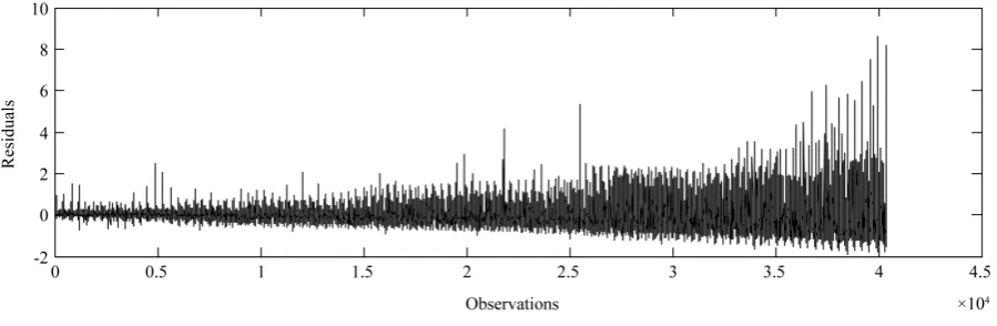
[image:5.595.89.539.561.708.2]Considering the case of simple Laspeyre price model described in Section 3, the first phase of computation involve the estimation of the parameter vector based on observed price data. We get the same values of esti-mates as Burney and Maqsood [7] obtained. The residuals versus observation numbers are plotted inFigure 1,
which shows the jumps along the constant central line. It has the longer ups and down as the time period in-creases proceeding far from the base period, however it exhibits the stationary situation. The value of Ljung-Box statistics is found to be 17,139, indicating the strong evidence towards second order serial correlation in series. We now estimate the autoregressive parameters of AR(2) process using Yule-walker method.Table 1 summa-rizes the results obtained in fitting AR(2) models. Akaike information criterion (AIC) of fitting AR(2) model is −1.7613, which is less than the AIC obtained in fitting AR(1) process. We have also checked for higher order of autoregressive processes but found no remarkable difference in values of AIC. Rather increasing the order of autoregressive process, it is recommended to choose a parsimonious model with comparatively less value of AIC.
The next phase certainly includes the extraction of influential observations using hat matrix and DFBETA measure. The diagonal hat values depend only on the weights of respective consumer items as shown in Equa-tion (10). We, therefore, get the same results as we acquired in Divisia index numbers (see Burney and Maqsood
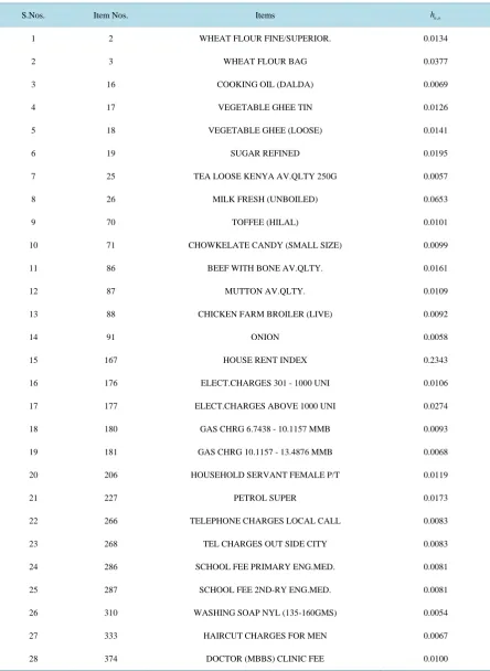
[26]). For the expediency of reader, the large quantities of hat entries that exceed the cut-off value 0.005348 are presented inTable 2. The highest hat value is parallel to house rent index, implying its importance in estimating the index numbers. Other leading items include milk fresh, wheat flour bag, and electric charges for the con-sumption of more than 1000 units.
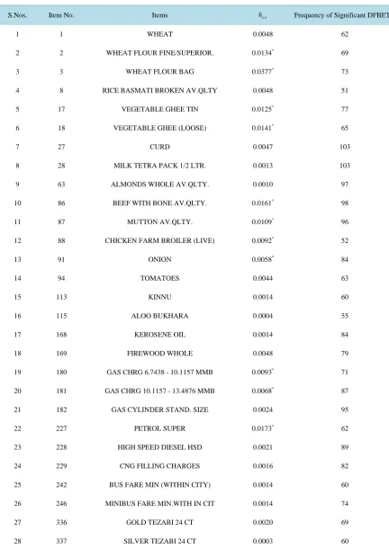
We compute DFBETA measure using Equation (11) for AR(2) process. The items that have more than 50 significant DFBETAs exceeding threshold point 0.009951 are listed in Table 3. The large hat values are represented by the values with superscript *. Several items have significant DFBETA values implying its influ-ence in estimating the simple Laspeyre price model. The reason behind this might be the comparison of current period prices to the fixed base period prices, and thus increasing the variation in prices as the difference between two periods rises. However, we may conclude here the first group food and beverages has the largest impact on estimation of parameter vector as 16 out of 28 items are from this group that influence more than 50 parameters in parameter vector. The curd and milk tetra pack with h27=0.0047, and h28=0.0013 respectively, may have a large impact on estimating index numbers relating to 103 months. In other words, these affect the values of 103 alphas in parameter vector. Other major significant commodity groups include fuel and lighting, and trans-portation and communication.
The house rent index with the highest h167=0.2343 have an influence on only eight regression estimate of
t
α . It might indicate that the items with large diagonal entries of hat matrix have not necessarily an influence on the parameter estimates.
5. Conclusions
In this paper, we considered the simple Laspeyre price model when the errors are generated from autoregressive process of order AR(2). We got the estimate of αt as the standard Laspeyre price index number formula. Next, we used the general form of hat matrix and DFBETA measure to extract the influential commodities in estimat-ing the Laspeyre price index number when the errors are serially correlated. The hat values are directly equal to the weights of respective items, implying that the greater the hat value, the more important commodity is, re-gardless of the values of autoregressive parameter. While, DFBETA measures are the functions of both hat val-ues and parameter of autoregressive process.
Lastly, an example was presented with reference to price data of Pakistan, which numerically confirms the results. From the findings of both hat values and DFBETA measure, the first commodity group of food and be-verages is the core group of items as the maximum number of items from this group has larger hat values and DFBETA measures. The wheat flour bag, milk fresh, meat with bones, electric consumption with more than 1000 units, and house rent index are the more crucial commodities that may have a larger impact on estimating the Laspeyre price index numbers.
Further motivation can be acquired on the techniques of influential cases of Laspeyre price index number
Table 1. Summary of fitting AR(2) process to the errors obtained in simple Laspeyre price model.
Simple Laspeyre Price Model with AR(2) Process
1 0.4733
Table 2. Significant hat values corresponding to commodities with AR(1) and AR(2) processes for simple Laspeyre price model.
S.Nos. Item Nos. Items hit it,
1 2 WHEAT FLOUR FINE/SUPERIOR. 0.0134
2 3 WHEAT FLOUR BAG 0.0377
3 16 COOKING OIL (DALDA) 0.0069
4 17 VEGETABLE GHEE TIN 0.0126
5 18 VEGETABLE GHEE (LOOSE) 0.0141
6 19 SUGAR REFINED 0.0195
7 25 TEA LOOSE KENYA AV.QLTY 250G 0.0057
8 26 MILK FRESH (UNBOILED) 0.0653
9 70 TOFFEE (HILAL) 0.0101
10 71 CHOWKELATE CANDY (SMALL SIZE) 0.0099
11 86 BEEF WITH BONE AV.QLTY. 0.0161
12 87 MUTTON AV.QLTY. 0.0109
13 88 CHICKEN FARM BROILER (LIVE) 0.0092
14 91 ONION 0.0058
15 167 HOUSE RENT INDEX 0.2343
16 176 ELECT.CHARGES 301 - 1000 UNI 0.0106
17 177 ELECT.CHARGES ABOVE 1000 UNI 0.0274
18 180 GAS CHRG 6.7438 - 10.1157 MMB 0.0093
19 181 GAS CHRG 10.1157 - 13.4876 MMB 0.0068
20 206 HOUSEHOLD SERVANT FEMALE P/T 0.0119
21 227 PETROL SUPER 0.0173
22 266 TELEPHONE CHARGES LOCAL CALL 0.0083
23 268 TEL CHARGES OUT SIDE CITY 0.0083
24 286 SCHOOL FEE PRIMARY ENG.MED. 0.0081
25 287 SCHOOL FEE 2ND-RY ENG.MED. 0.0081
26 310 WASHING SOAP NYL (135-160GMS) 0.0054
27 333 HAIRCUT CHARGES FOR MEN 0.0067
Table 3. Frequency of significant DFBETA for αtcorresponding to items and their hat values for simple Laspeyre price
model.
S.Nos. Item No. Items hit it, Frequency of Significant DFBETA
1 1 WHEAT 0.0048 62
2 2 WHEAT FLOUR FINE/SUPERIOR. 0.0134* 69
3 3 WHEAT FLOUR BAG 0.0377* 73
4 8 RICE BASMATI BROKEN AV.QLTY 0.0048 51
5 17 VEGETABLE GHEE TIN 0.0125* 77
6 18 VEGETABLE GHEE (LOOSE) 0.0141* 65
7 27 CURD 0.0047 103
8 28 MILK TETRA PACK 1/2 LTR. 0.0013 103
9 63 ALMONDS WHOLE AV.QLTY. 0.0010 97
10 86 BEEF WITH BONE AV.QLTY. 0.0161* 98
11 87 MUTTON AV.QLTY. 0.0109* 96
12 88 CHICKEN FARM BROILER (LIVE) 0.0092* 52
13 91 ONION 0.0058* 84
14 94 TOMATOES 0.0044 63
15 113 KINNU 0.0014 60
16 115 ALOO BUKHARA 0.0004 55
17 168 KEROSENE OIL 0.0014 84
18 169 FIREWOOD WHOLE 0.0048 79
19 180 GAS CHRG 6.7438 - 10.1157 MMB 0.0093* 71
20 181 GAS CHRG 10.1157 - 13.4876 MMB 0.0068* 87
21 182 GAS CYLINDER STAND. SIZE 0.0024 95
22 227 PETROL SUPER 0.0173* 62
23 228 HIGH SPEED DIESEL HSD 0.0021 89
24 229 CNG FILLING CHARGES 0.0016 82
25 242 BUS FARE MIN (WITHIN CITY) 0.0014 60
26 246 MINIBUS FARE MIN.WITH IN CIT 0.0014 74
27 336 GOLD TEZABI 24 CT 0.0020 69
[image:8.595.93.526.106.717.2]model by extending the approach with autoregressive processes of higher lags and then using the same methods described in Section 3 and Section 4. Moreover, it opens many opportunities to work with other index numbers, particularly for those, which are used to show the current consumption pattern of consumers instead of relying on fixed base approach.
Acknowledgements
The authors are thankful to Dept. of Computer Science and Dept. of Statistics University of Karachi for provid-ing computprovid-ing and research facilities.
References
[1] Maqsood, A. and Burney, S.M.A. (2008) Study of Inflation in Pakistan Using Statistical Approach. 4th International
Statistical (ISSOS), University of Gujrat, Hafiz Hayat Campus, Pakistan.
[2] Clements, K.W. and Izan, H.Y. (1981) A Note on Estimating Divisia Index Numbers. International Economic Review,
22, 745-747. http://dx.doi.org/10.2307/2526174
[3] Clements, K.W. and Izan, H.Y. (1987) The Measurement of Inflation: A Stochastic Approach. Journal of Business and
Economic Statistics, 5, 339-350.
[4] Selvanathan, E.A. (1991) Standard Errors for Laspeyers and Paasche Index Numbers. Economics Letters, 35, 35-38.
http://dx.doi.org/10.1016/0165-1765(91)90101-P
[5] Selvanathan, E.A. (1993) More on the Laspeyers Price Index. Economics Letters, 43, 157-162.
http://dx.doi.org/10.1016/0165-1765(93)90029-C
[6] Selvanathan, E.A. (2003) Extending the Stochastic Approach to Index Numbers: A Comment. Applied Economics
Let-ters, 10, 213-215. http://dx.doi.org/10.1080/1350435022000043986
[7] Burney, S.M.A. and Maqsood, A. (2013) Extending the Stochastic Approach to Paasches Price Index Numbers.
Pakis-tan Journal of Engineering Technology & Science, 3, 1-17.
[8] Prais, G.J. and Winsten, C.B. (1954) Trend Estimates and Serial Correlation. Cowles Commission Discussion Paper,
Stat. No. 383, University of Chicago, Chicago.
[9] Kadiyala, K.R. (1968) A Transformation Used to Circumvent the Problem of Autocorrelation. Econometrica, 36, 93-
96. http://dx.doi.org/10.2307/1909605
[10] Griliches, Z. and Rao, P. (1969) Small-Sample Properties of Several Two-Stage Regression Methods in the Context of
Autocorrelated Disturbances. Journal of American Statistical Association, 64, 253-272.
http://dx.doi.org/10.1080/01621459.1969.10500968
[11] Maeshiro, A. (1979) On the Retention of the First Observation in Serial Correlation Adjustment of Regression Models.
International Economic Review, 20, 259-265. http://dx.doi.org/10.2307/2526430
[12] Park, R.E. and Mitchell, B.M. (1980) Estimating the Autocorrelated Error Model with Trended Data. Journal of
Eco-nometrics, 13, 185-201. http://dx.doi.org/10.1016/0304-4076(80)90014-7
[13] Belsley, P.A., Kuh, E. and Welsch, R.E. (1980) Regression Diagnostics. John Wiley, New York.
http://dx.doi.org/10.1002/0471725153
[14] Cook, R.D. (1977) Detection of Influential Observations in Linear Regression. Technometrics, 19, 15-18.
http://dx.doi.org/10.2307/1268249
[15] Cook, R.D. (1979) Influential Observations in Linear Regression. Journal of American Statistical Association, 74, 169-
174. http://dx.doi.org/10.1080/01621459.1979.10481634
[16] Cook, R.D. and Weisberg, S. (1982) Residuals and Influence in Regression. Chapman and Hall, New York.
[17] Draper, N.R. and John, J.A. (1981) Influential Observations and Outliers in Regression. Technometrics, 23, 21-26.
http://dx.doi.org/10.1080/00401706.1981.10486232
[18] Draper, N.R. and Smith, H. (1998) Applied Regression Analysis. 3rd Edition, John Wiley, New York.
[19] Puterman, M.L. (1988) Leverage and Influence in Autocorrelated Regression Model. Journal of the Royal Statistical
Society, 37, 76-86.
[20] Cochrane, D. and Orcutt, G.H. (1949) Application of Least Squares Regression to Relationships Containing Auto-Cor-
related Error Terms. Journal of the American Statistical Association, 44, 32-61.
[21] Stemann, D. and Trenkler, G. (1993) Leverage and Cochrane-Orcutt Estimation in Linear Regression. Communications
[22] Pena, D. (2005) A New Statistic for Influence in Linear Regression. Technometrics, 47, 1-12.
http://dx.doi.org/10.1198/004017004000000662
[23] Turkan, S. and Toktamis, O. (2012) Detection of Influential Observations in Ridge Regression and Modified Ridge
Regression. Model Assisted Statistics and Applications, 7, 91-97.
[24] Turkan, S. and Toktamis, O. (2013) Detection of Influential Observations in Semiparametric Regression Model. Re-
vista Colombiana de Estadistica, 36, 91-97.
[25] Barry, A.M., Burney, S.M.A. and Bhatti, M.I. (1997) Optimum Influence of Initial Observations in Regression Models
with AR(2) Errors. Applied Mathematics and Computation, 82, 57-65.
http://dx.doi.org/10.1016/S0096-3003(96)00024-0
[26] Burney, S.M.A. and Maqsood, A. (2014) Influential Observations in Stochastic Model of Divisia Index Numbers with
AR(1) Errors. Applied Mathematics, 5, 975-982. http://dx.doi.org/10.4236/am.2014.56093
[27] Wise, J. (1955) The Autocorrelation Function and the Spectral Density Function. Biometrika, 42, 151-159.
http://dx.doi.org/10.2307/2333432
[28] Pakistan Bureau of Statistics. Monthly Bulletin of Statistics.