Atmospheric and Climate Sciences, 2014, 4, 272-289
Published Online April 2014 in SciRes. http://www.scirp.org/journal/acs http://dx.doi.org/10.4236/acs.2014.42029
Climate Change in La Plata Basin as Seen by
a High-Resolution Global Model
Mario N. Nuñez1,2,3, Josefina Blázquez1,2,3
1Centro de Investigaciones del Mar y la Atmósfera (CIMA-CONICET/FCEN-UBA), Buenos Aires, Argentina 2Instituto Franco Argentino del Clima y sus Impactos (UMI IFAECI/CNRS), Buenos Aires, Argentina 3Departamento de Ciencias de la Atmósfera y los Océanos (FCEN-UBA), Buenos Aires, Argentina
Email: [email protected], [email protected]
Received 20 December 2013; revised 15 January 2014; accepted 23 January 2014
Copyright © 2014 by authors and Scientific Research Publishing Inc.
This work is licensed under the Creative Commons Attribution International License (CC BY).
http://creativecommons.org/licenses/by/4.0/
Abstract
This paper analyses the climate change in La Plata Basin, one of the most important regions in South America due to its economy and population. For this work it has been used the Meteorologi- cal Research Institute (MRI) and the Japanese Meteorological Agency (JMA) atmospheric global model. For both near and far future, the projected changes for temperature over the entire basin were positive, although they were only statistically significant at the end of the XXI century. Changes in the annual cycle of mean temperature were also positive in all subregions of the basin. Regarding precipitation, there were no changes in the near future that were statistically signifi- cant. The summer (winter) is the only season where both models project positive (negative) changes for both periods of the future. In the transitional seasons these changes vary depending on the spatial resolution model and the area of study. The annual cycle showed that the largest changes in precipitation (positive or negative) coincide with the rainy season of each subregion. Regarding the interannual variability of temperature, it was found that the 20 km. model pro- jected a decrease of this variability for both near and far future, especially in summer and autumn. On the other hand, the 60 km. ensemble model showed a decreased of year-to-year variability for summer and an increase in winter and spring. It was also found that both models project an in- crease in precipitation variability for winter and summer, while in other seasons, only the 60 km. ensemble model presents the mentioned behavior.
Keywords
Climate Change; La Plata Basin; High Resolution Global Model; Projections
1. Introduction
a global high-resolution climate model is presented. The global model of Meteorological Research Institute (MRI) and Japanese Meteorological Agency (JMA) is used in this study.
In recent years there are few studies in the literature describing the present climate and future projections of the La Plata Basin using climate models (global or regional). Among them, [1] evaluated how a set of global models (one generation before the CMIP3) represents the present climate of the La Plata Basin and they found that the simulated precipitation does not match well with the observed data (some underestimations were found over eastern Argentina, Uruguay and southern Brazil). In the same region, these authors also found that the models overestimate the observed temperature. Furthermore, [2] evaluated the ability of some models of the WCRP-CMIP3 program to represent the temperature and precipitation in the present climate in the La Plata Ba- sin and projected changes for the future. Regarding the temperature they found that the observed amplitude be- tween summer and winter is overestimated by the ensemble of models, especially on the centre and south of the La Plata Basin. They also found some deficiencies in the representation of precipitation over La Plata Basin, such as overestimation of intense precipitation events (weak) on the north (central and southern) basin. When the mentioned authors analyzed precipitation projections, it was found positive changes in autumn and winter on the northern sub regions of the basin, as well as in the south and centre throughout the year. The rainfall distri- bution showed an increase (decrease) in the frequency of weak (intense) events rainfall in the north of the basin and an opposite change in the centre and south of it. Moreover, within the project CLARIS-LPB (Europe-South America Network for Climate Change Assessment and Impact Studies in La Plata Basin) seven high-resolution regional experiments have recently conducted over South America, with emphasis on the La Plata Basin. These simulations were performed in order to obtain detailed projections in the region considering a possible climate change scenario (some preliminary results could be found in [3]. Besides, [4] evaluated how these models rep- resent the present climate over South America. These authors found that in general all models adequately de- scribe the spatial characteristics of precipitation and temperature, although they detected some defects in the representation of annual and seasonal cycle, especially in precipitation (underestimation of precipitation during the winter on Uruguay and during January, February and March on Low-Parana sub-basin).
On the other hand, there are loads of studies that analyse the climate change over South America using dif- ferent models ([5]-[8]; among others). If the focus is put in LPB region, in general all of the mentioned authors agree in projecting for the XXI century an increase of temperature in all the seasons, a positive change of pre- cipitation in summer and a negative in winter. But, as it was said previously there is few papers studying climate change over LPB region in detail.
This work is a part of a previous study that includes all of South America [5]. We improve here the study only over La Plata Basin because its economic importance and large population. Most of the generation of power electricity for Argentina, Brazil Paraguay and Uruguay come from La Plata River and its tributaries: Paraná, Paraguay and Uruguay rivers.La Plata Basin is the largest water system in South America after the Amazon watershed and the fifth largest in the world. The basin includes important territories belonging to the central and northern Argentina, southern/southeastern Brazil, southern and eastern Bolivia, most of Uruguay, and the whole territory of Paraguay, and is home to about 50% of their combined population, generating about 70% of their to- tal Gross National Product. The principal sub-basins are those of the Paraná, Paraguay and Uruguay rivers and the average flow of the basin is 23.000 m3/s.
Numerous studies have focused on studying the evolution of the climate of recent years on the La Plata Basin. Regarding the trends in precipitation, [9] and [10] found that in the last 40 years the rainfall has increased by 10% over the basin, reaching values of 30% in some areas. Moreover, the frequency of rain events that exceed 100 mm in central and eastern Argentina has tripled in recent years [11]. This increase in rainfall has led to positive changes in the river flow ([12]-[14]) since the evaporation due to temperature increase in the region has not changed significantly ([15] [16]). However, in some areas of the basin (i.e. Paraguay sub-basin) part of the in- crease in runoff can be attributed to land-use change (deforestation), especially since 1970 [17]. Because of this, the activities dependent on water resources would be affected enough to changes in precipitation and temperature that could lead to a possible climate change in the coming years. According to [11], the most adverse effect of climatic changes in the region is the increased frequency and severity of floods, which in recent years have been increasing as a result of both climatic and hydrological trends, such as the occupation urban and agricultural areas at risk of flooding.
M. N. Nuñez, J. Blázquez
MRI model and observations over LPB region was assessed in [19]. A summary of the results are present below. In general terms, the spatial patterns of temperature and precipitation are well represented by the MRI/JMA model. To study the basin in detail, it was divided in sub-regions. The phase of the annual cycle of air tempera- ture is well represented instead the amplitude is greater than observed in some sub-regions (Paraguay, Up- Parana and SACZ). Regarding the annual cycle of precipitation the amplitude is overestimated in Paraguay, while in Uruguay and Up-Parana was underestimated by the model. The observed interannual variability of temperature over the basin was lower than 1.5˚C and it was found that the 20 km resolution model overestimated the year-to-year variability in all the sub-regions, while the ensemble of 60 km resolution model represents it adequately. On the other hand, the precipitation variability is well represented by the MRI/JMA model. Finally, it was found a cold bias in the 20 km resolution model (values lower than −1.5˚C) in some sub-regions and sea- sons and a warm bias (reaching 3˚C) in most of the sub-regions and seasons of ensemble of 60 km resolution model. In precipitation, both resolution models behave similar, showing a wet bias in Paraguay (with values reaching 2 mm/day) and a dry bias in the rest of the sub-regions (with values lower than −1 mm/day).
This paper will address possible scenarios of climate change over La Plata Basin, produced by the MRI/JMA global model.
2. Model and Experiment Design
The global model MRI/JMA is used in this study. It is a global atmospheric model with a horizontal grid size of about 20 km (TL959) and 60 levels (L60) in the vertical with the model top at 0.1 hPa. The model is hydrostatic, and uses a prognostic Arakawa-Schubert scheme,the [20] and [21] boundary layer parameterization; the land surface is described by the Simple Biosphere (SiB) model following [22] and [23]. For more details on model setup see [24].
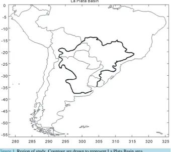
For the simulation scenarios, greenhouse gas emissions are specified from SRESA1B emission scenario (Spe- cial Report on Emissions Scenarios, [25]) and it was used to run the coupled model that was used as boundary conditions in the atmospheric model. It is widely know that there are more emission scenarios available to run models, but in this case it was chosen a medium scenario. Consequently it is important to keep in mind that this choice could bring to uncertainties in the projections, especially in the case of temperature [26] [27]. Figure 1 dis- plays the region used to analyse the results in this study. The experiments are described in Table 1. The time slice technique was used to perform the experiments. The slices was divided as following: present (1979-2003), near future (2015-2039) and far future (2075-2099). The model was run with two different resolutions (20 km and 60 km). In the Near and far future simulations initial condition was built using CMIP3 multimodel ensemble (SNF, SF, HNF, HF), CSIRO-MK3.0 model (HNF_csiro, HF_csiro), MIROCH3.2 model (HNF_miroch, HF_miroch) and MRI-GCM2.3.2 model (HNF_mri, HF_mri). These models belong to the WCRP-CMIP3 Pro- gram [28]. In the case of the 60 km experiments, the three members were constructed by changing the initial date in the three different years. So, for the 60 km experiments the ensemble average was performed with 12 members. It is worth to clarify that just one simulation was performed with 20 km super high resolution model. Due to this model is not a coupled atmospheric ocean model, the SST for near future and future simulations was constructed using an estimation method. For details of the SST preparation see Section 2.2 of [29].
3. Results
3.1. Changes in the Mean Climate
3.1.1. Temperature
Table 1. Experimental design.
Experiment name Period Initial condition Number of members
SRNF 2015-2039 CMIP3 multimodel ensemble1 1
SRF 2075-2099 CMIP3 multimodel ensemble1 1
HRNF 2015-2039 CMIP3 multimodel ensemble1 3
HRF 2075-2099 CMIP3 multimodel ensemble1 3
HRNF_csiro 2015-2039 CSIRO-MK3.02 3
HRF_csiro 2075-2099 CSIRO-MK3.02 3
HRNF_miroch 2015-2039 MIROCH3.2 (hires)3 3
HRF_miroch 2075-2099 MIROCH3.2 (hires)3 3
HRNF_mri 2015-2039 MRI‐CGCM2.3.24 3
HRF_mri 2075-2099 MRI‐CGCM2.3.24 3
SR means “super-high resolution” (20 km) and HR “high resolution” (60 km). NF and F mean “Near Future” and “Future” respectively. 1Coupled Model Intercomparison Project, third phase; 2Commonwealth Scientific and Industrial Research Organisation, Atmospheric Research, Australia; 3Center for Climate System Research (University of Tokyo), National Institute for Environmental Studies, and Frontier Research Center for Global Change of Japan Agency for Marine Earth Science and Technology, Japan; 4Meteorological Research Institute, Japan.
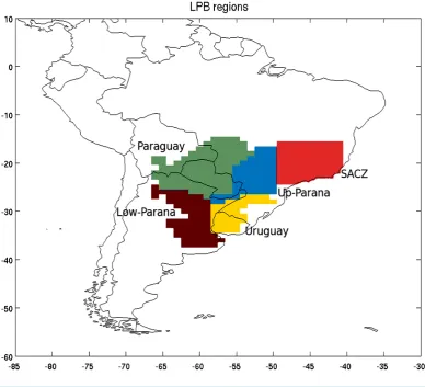
Figure 1. Region of study. Countour are drawn to represent La Plata Basin area.
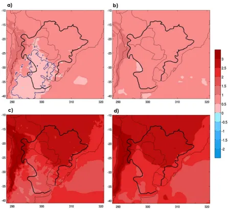
significant (Figure 2(a) and Figure 2(b)).This could be related to the fact that the high resolution model is based on a single run.Figure 3 shows the projected changes for the average temperature during fall, for the near future and for the end of the century, using both experiments. For the near future, both models project changes less than 1˚C, while at the end of the century, the changes reach values between 2.5˚C and 3˚C (1.5˚C and 2.5˚C) over north (south) of the basin. When comparing both models in the near future, it again shows that the 20 km model resolution produces no significant changes over south of the basin, while the ensemble model exhibits significant changes with a confidence level of 90% over the entire study region.
M. N. Nuñez, J. Blázquez
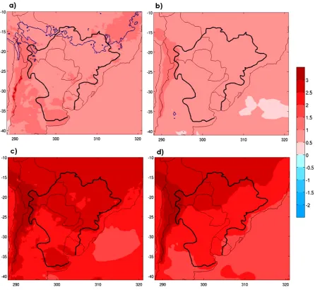
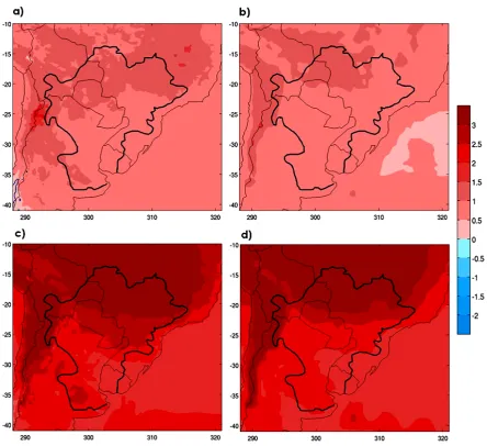
Figure 2. Mean surface air temperature change for summer (˚C). (a) Near future minus present, for the 20 km model resolution; (b) Near future minus present, for the 60 km ensemble model; (c) Far future minus present, for the 20 km model resolution; (d) Far future minus present, for the 60 km ensemble model. Black contour indicates La Plata Basin region. The regions inside blue contours indicate 90% confidence level. Student t-test. Figures with no blue contours mean that the entire region is statistitcal significant.
north/northeast of the basin. If both experiments are compared, one can see that in the near future the two mod- els project significant changes only over the northern part of the region.
Figure 5shows the changes in the average surface temperature for the spring season. Both models have val- ues between 0.5˚C and 1.5˚C in the near future and greater than 3˚C (2˚C) at the end of the XXI century over the northern (southern) portions of the basin. In this season all the changes are significant at a confidence level of 90%.
[image:5.595.92.539.85.495.2]Figure 3. Mean surface air temperature change for fall (˚C). (a) Near future minus present, for the 20 km model resolution; (b) Near future minus present, for the 60 km ensemble model; (c) Far future minus present, for the 20 km model resolution; (d) Far future minus present, for the 60 km ensemble model. Black contour indicates La Plata Basin region. The regions inside blue contours indicate 90% confidence level. Student t-test. Figures with no blue contours mean that the entire region is statistitcal significant. Region of study. Countour are drawn to represent La Plata Basin area.
distant future for both models. Meanwhile, changes between 0.5˚C and 2˚C are shown for the near future. The changes in the annual cycle, at the end of this century are significant at a confidence level of 90%. However, in the near future there are some months in some sub regions (indicated in the figure with a circle) where the changes were not statistically significant. Such behaviour is observed especially in the ensemble produced by the 60 km resolution model.
3.1.2. Precipitation
M. N. Nuñez, J. Blázquez
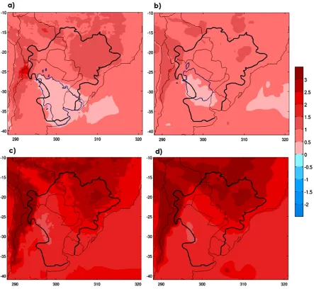
Figure 4. Mean surface air temperature change for winter (˚C). (a) Near future minus present, for the 20 km model resolution; (b) Near future minus present, for the 60 km ensemble model; (c) Far future minus present, for the 20 km model resolution; (d) Far future minus present, for the 60 km ensemble model. Black contour indicates La Plata Basin region. The regions inside blue contours indicate 90% confidence level. Student t-test. Figures with no blue contours mean that the entire region is statistitcal significant. Region of study. Countour are drawn to represent La Plata basin area.
the maximum seen in the 60 km model is shifted to the north if it is compared with CNRM model. In this case, the changes are statistically significant (with a confidence level of 90%) in some areas of the basin, depending on the model considered. For the high-resolution model there are statistically significant changes in the centre and north of the basin (Figure 8(c)), while for the 60 Km. ensemble model significant values are in the west and centre of the study region (Figure 8(d)).
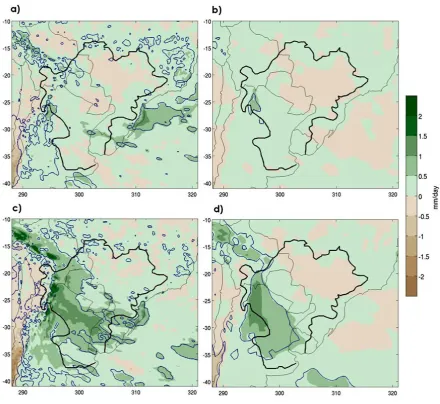
Changes in precipitation projected during fall, both in the near future and in the far future are shown in Figure 9. In the near future, both models project changes positive and negative in the south to the north of the basin (from 0 to ±0.5 mm/day), while at the end of the century, the 20 km resolution model projected positive changes over most of the basin (reaching values of 1.5 mm/day to the southwest of it). In addition, the ensemble model pro-jected negative changes (near −0.5 mm/day) in the north and positive (between 0.5 and 1.5 mm/day) in the southwest of the study region. Both models show, for the end of the century, statistical significance of the changes projected in the southwest of the basin.
[image:7.595.93.537.86.494.2]Figure 5. Mean surface air temperature change for spring (˚C). (a) Near future minus present, for the 20 km model resolu- tion; (b) Near future minus present, for the 60 km ensemble model; (c) Far future minus present, for the 20 km model resolution; (d) Far future minus present, for the 60 km ensemble model. Black contour indicates La Plata Basin region. The regions inside blue contours indicate 90% confidence level. Student t-test. Figures with no blue contours mean that the entire region is statistitcal significant. Region of study. Countour are drawn to represent La Plata basin area.
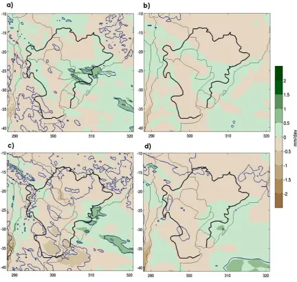
negative (−0.5 mm/day) over the entire basin, especially in the far future. Negative changes in winter were pro- jected also by some of WCRP-CMIP3 models [31]. During this season, only the 20 km resolution model pre- sented statistically significant changes in some areas of the basin in the late XXI century.
Finally, the projected precipitation changes with both models for spring are shown in Figure 11. In the near future, the model of 20 km (Figure 11(a)), projected positive changes in most of the basin reaching values of 1 mm/day over southern Paraguay and Misiones province. Instead, the ensemble model of 60 km (Figure 11(b)) shows changes slightly negative (positive) on the southwest (northeast) of the study region. It is worth mention- ing that none of these changes is statistically significant (considering a confidence level of 90%). By the end of the century, both models show a similar behaviour: positive change values of precipitation over the central and eastern basin (reaching values of 2 mm/day) and a slightly negative change to the south of it. In addition, posi- tive projected changes are statistically significant in both models.
M. N. Nuñez, J. Blázquez
Figure 6. The sub-regions inner La Plata Basin considered in the present study.
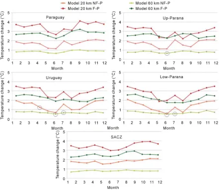
regions shown in Figure 6. It can be seen that the largest changes (positive or negative) are projected for the summer, fall and spring. These months coincide in most of the sub regions, with the rainy season. In particular, the figure also shows that the sub regions Paraguay, Low-Paraná and SACZ show very small changes (which are generally negative) during winter and major positive changes during the summer and fall. On the other hand, the remaining regions (Up-Parana and Uruguay) show positive changes in the annual cycle in almost every month of the year. It is worth mentioning that the projected changes in the annual cycle experiments with the model MRI/ JMA are not statistically significant in most sub regions and months. The figure shows some exceptions; generally occur in the spring, summer and fall.
3.2. Changes in the Interannual Variability
[image:9.595.118.507.88.441.2]In this section we analyse the changes in the interannual variability of temperature and precipitation over the sub regions of Plata Basin defined inFigure 6.
Figure 13shows the standard deviation for the seasonal temperature simulated by the model MRI/JMA (in both resolutions) for near and far future. The figure shows that in all seasons, the 20 km resolution model projected a decrease of interannual variability for the future (near and far). This feature is seen mainly during summer and fall. Instead, the 60 km ensemble model shows an increase (decrease) of that variability for the winter and spring (summer) in most of the analyzed sub regions.
Figure 7. Changes in the annual cycle of mean temoerature (˚C) for the sub-regions defined in Figure 6. Filled circles indicate far future minus present. Asterisks indicate present near future minus present. The orange lines represent the results for the 20 km model and green lines represent the ensemble model of 60 km. The black circles indicate the months in which the change is not statistically significant considering a confidende level of 90%. Student t-test .
model projected slightly negative changes in the majority of the sub-regions.
As discussed in [5], the reason for the minor changes in year-to-year variability may be the way initial condi- tions (SST and sea ice) for the future model runs were built. The present climate variability is used to initialise the future experiments. On the other hand, it is widely known that climate variability in many parts of the study area is largely determined by the variability of SST in the tropical equatorial Pacific Ocean caused by the ENSO phenomenon (El Niño-Southern Oscillation) ([32]-[34]; among others). So, on the one hand it has been proved that variability in SST (especially in tropical areas) is strongly associated with the climate variability of LPB re- gion, on the other, the future initial conditions of the model (for example, SST) were built taking into account the present variability. This could explain the small change in precipitation and temperature interannual variabil- ity that the MRI/JMA model projects in La Plata Basin.
4. Summary and Conclusions
This paper presents the results from global simulations of climate change under the IPCC emission scenario A1B for near future and for the end of the XXI century. These results are applied to the region of the La Plata Basin in southern South America.
M. N. Nuñez, J. Blázquez
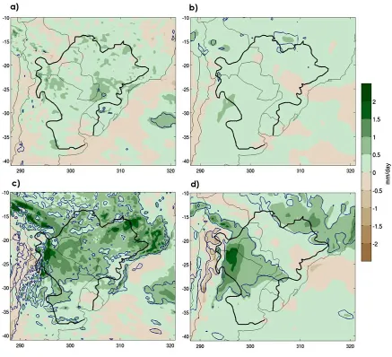
Figure 8. Mean precipitation change for summer (mm/day). (a) Near future minus present, for the 20 km model resolution; (b) Near future minus present, for the 60 km ensemble model; (c) Far future minus present, for the 20 km model resolution; (d) Far future minus present, for the 60 km ensemble model. Black contour indicates La Plata Basin region. The regions inside blue contours indicate 90% confidence level. Student t-test. Figures with no blue contours mean that the entire region is statistitcal significant. Region of study. Countour are drawn to represent La Plata basin area.
were performed with the JMI/MRI global model. The focus of the present paper was studying the changes in the surface variables, air temperature and precipitation. Changes in the year-to-year variability were also analysed. Our primary conclusions can be summarized as follows:
1) In all seasons, La Plata Basin undergoes a warming in the A1B scenario for the near future and to the end of the present century. The warming is in the range of 0.5˚C - 1.5˚C for the near future and 1.5˚C - 2.5˚C for the end of the century. Maximum changes in the mean temperature are projected for the northern La Plata Basin during all seasons. For the far future the changes in the mean temperature are statistically significant at 90% sig- nificance level for both model resolutions. However, in the near future the significance depends on the season and the considered experiment. The annual cycle of mean temperature also reflects the positive changes found previously. In all sub regions studied, projected changes in the annual cycle are between 2˚C and 4˚C for the distant future, and between 0.5˚C and 2˚C for the near future. Most of these changes are statistically significant at 90% confidence level.
Figure 9. Mean precipitation change for fall (mm/day). (a) Near future minus present, for the 20 km model resolution; (b) Near future minus present, for the 60 km ensemble model; (c) Far future minus present, for the 20 km model resolution; (d) Far future minus present, for the 60 km ensemble model. Black contour indicates La Plata Basin region. The regions inside blue contours indicate 90% confidence level. Student t-test. Figures with no blue contours mean that the entire region is statistitcal significant. Region of study. Countour are drawn to represent La Plata Basin area.
[image:12.595.96.537.84.488.2]M. N. Nuñez, J. Blázquez
Figure 10. Mean precipitation change for winter (mm/day). (a) Near future minus present, for the 20 km model resolution; (b) Near future minus present, for the 60 km ensemble model; (c) Far future minus present, for the 20 km model resolution; (d) Far future minus present, for the 60 km ensemble model. Black contour indicates La Plata Basin region. The regions inside blue contours indicate 90% confidence level. Student t-test. Figures with no blue contours mean that the entire region is statistitcal significant. Region of study. Countour are drawn to represent La Plata basin area.
coinciding with the rainy season of each sub region. Most of these changes were not statistically significant. 3) Changes in the interannual variability of temperature and precipitation were also studied on the sub regions defined in the basin. The 20 km resolution model showed a decrease of temperature variability for the future, especially during the summer and fall. Conversely, the 60 km ensemble model showed an increase (decrease) of this variability for the winter and spring (summer) in most of the sub regions considered. For the interannual variability of precipitation, both models projected a slight increase of this variability for summer and winter, while for the transitional seasons; only ensemble 60 km projected model projected a similar behaviour in most sub regions studied.
Figure 11. Mean precipitation change for spring (mm/day). (a) Near future minus present, for the 20 km model resolution; (b) Near future minus present, for the 60 km ensemble model; (c) Far future minus present, for the 20 km model resolution; (d) Far future minus present, for the 60 km ensemble model. Black contour indicates La Plata Basin region. The regions inside blue contours indicate 90% confidence level. Student t-test. Figures with no blue contours mean that the entire region is statistitcal significant. Region of study. Countour are drawn to represent La Plata basin area.
Finally, some preliminary considerations about runoff could be done with these results. The increased pre- cipitation for the future (which is also observed in the present) and the expected increase in evaporation [29], due to increase of temperature over the basin could lead to increased runoff in the rivers of the La Plata Basin. In fact this model projects a positive change in runoff (approaching it like the difference between precipitation and evaporation [5]). So, as a result of balance between precipitation, evaporation and runoff over the basin, it could lead to an increase in the rivers runoff impacting positively on the hydropower generation. On the other hand, it is important to note that the previous analysis was done without taking into account some other processes that maybe could influence the runoff (like land use or occupation of land). Besides, this statement has to be taken into account carefully, because these results correspond only to one model. To have a better understanding of this topic, multi-model simulations and their associated uncertainty have to be analysed.
Acknowledgements
M. N. Nuñez, J. Blázquez
Figure 13. Standard deviation of seasonal surface temperature (˚C) averaged over all the sub-regions defines in Figure 6. In red, results for the 20 km model. In green, for the 60 km ensemble model. Squares indicate present simulations, circles simulations of the near future and triangles for far future.
Figure 14. Coefficient of variation of seasonal precipitation (mm/day) averaged over all the sub-regions defines inFigure 6. In red, results for the 20 km model. In green, for the 60 km ensemble model. Squares indicate present simulations, circles simulations of the near future and triangles for far future.
Programme (FP7/2007-2013), under Grant Agreement N˚212492. CLARIS LPB. A Europe-South America Network for Climate Change Assessment and Impact Studies in La Plata Basin.
References
[image:16.595.92.537.277.600.2]M. N. Nuñez, J. Blázquez
[2] Silvestri, G., Vera, C., Jacob, D., Pfeifer, S. and Teichmann, C. (2008) A High-Resolution 43-Year Atmospheric Hind- cast for South America Generated with the MPI Regional Mode. Climate Dynamics, 32, 693-709.
http://dx.doi.org/10.1007/s00382-008-0423-5
[3] Samuelson, P., Solman, S., Sanchez, E., Rocha, R., Li, L., Marengo, J., Remedio, A. and Berbery, H. (2013) Regional Climate Change Projections over South America Based on the CLARIS-LPB RCM Ensemble. Geophysical Research Abstracts, 15, EGU2013-5800.
[4] Solman, S.A., Sánchez, E., Samuelsson, P., da Rocha, R.P., Li, L., Marengo, J., Pessacg, N., Remedio, A.R.C., Chou, S.C., Berbery, H., Le Treut, H., de Castro, M. and Jacob, D. (2013) Evaluation of an Ensemble of Regional Climate Model Simulations over South America Driven by the ERA-Interim Reanalysis: Model Performance and Uncertainties. Climate Dynamics, 41, 1139-1157. http://dx.doi.org/10.1007/s00382-013-1667-2
[5] Blázquez, J., Nuñez, M.N. and Kusunoki, S. (2012) Climate Projections and Uncertainties over South America from MRI/JMA Global Model Experiments. Atmospheric and Climate Sciences, 2, 381-400.
http://dx.doi.org/10.4236/acs.2012.24034
[6] Marengo, J.A., Chou, S.C., Kay, G., Alves, L.M., Pesquero, J.F., Soares, W.R., Santos, D.C., Lyra, A.A., Sueiro, G., Betts, R., Chagas, D.J., Gomes, J.L., Bustamante, J.F. and Tavares, P. (2012) Development of Regional Future Climate Change Scenarios in South America Using the Eta CPTEC/HadCM3 Climate Change Projections: Climatology and Regional Analyses for the Amazon, Sao Francisco and the Parana River Basins. Climate Dynamics, 38, 1829-1848.
http://dx.doi.org/10.1007/s00382-011-1155-5
[7] Cabré, M.F., Solman, S. and Nuñez, M.N. (2010) Creating Regional Climate Change Scenarios over Southern South America for the 2020’s and 2050’s Using the Pattern Caling Technique: Validity and Limitations. Climatic Change, 98, 449-469. http://dx.doi.org/10.1007/s10584-009-9737-5
[8] Nuñez, M.N., Solman, S.A. and Cabré, M.F. (2009) Regional Climate Change Experiments over Southern South America. II: Climate Change Scenarios in the Late Twenty-First Century. Climate Dynamics, 32, 1081-1095.
http://dx.doi.org/10.1007/s00382-008-0449-8
[9] Castañeda, M.E. and Barros, V. (1994) Las tendencias de la precipitación en el Cono sur de América al Este de los Andes. Meteorológica, 19, 23-32.
[10] Minetti, J., Vargas, W., Poblete, A., Acuña, L. and Casagrande, G. (2003) Non-Linear Trends and Low Frequency Os- cillations in Annual Precipitation over Argentina and Chile, 1931-1999. Atmósfera, 16, 119-135.
[11] Barros, V. (2006) Introducción. Capítulo I. In: Barros, V., Clarke, R. and Silva Días, P., Eds., El Cambio Climático en la Cuenca del Plata, CIMA, Buenos Aires, 230 p.
[12] García, N. and Vargas, W. (1998) The Temporal Climatic Variability in the Rio De La Plata Basin Displayed by the River Discharges. Climatic Change, 38, 359-379. http://dx.doi.org/10.1023/A:1005386530866
[13] Genta, J.L., Perez Iribarne, G. and Mechoso, C. (1998) A Recent Increasing Trend in the Streamflow of Rivers in Southeastern South America. Journal of Climate, 11, 2858-2862.
http://dx.doi.org/10.1175/1520-0442(1998)011<2858:ARITIT>2.0.CO;2
[14] Camilloni, I. (2005) Variabilidad y tendencias hidrológicas en la Cuenca del Plata. Capítulo 3. In: Barros, V., Men- éndez, A. and Nagy, G., Eds., El Cambio Climático en el Río de la Plata, CIMA, Buenos Aires, 200 p.
[15] Berbery, E.H. and Barros, V.R. (2002) The Hydrologic Cycle of the La Plata Basin in South America. Journal of Hy- drometeorology, 3, 630-645. http://dx.doi.org/10.1175/1525-7541(2002)003<0630:THCOTL>2.0.CO;2
[16] Baéz, J. (2006) Tendencias en la evaporación. Capítulo VII. In: Barros, V., Clarke, R. and Silva Días, P., Eds., El Cambio Climático en la Cuenca del Plata, CIMA, Buenos Aires, 230 p.
[17] Collischonn, W., Tucci, C.E.M. and Clarke, R.T. (2001) Further Evidence of Changes in the Hydrological Regime of the River Paraguay: Part of a Wider Phenomenon of Climate Change? Journal of Hydrology, 245, 218-238.
http://dx.doi.org/10.1016/S0022-1694(01)00348-1
[18] Blázquez, J. and Nuñez, M.N. (2013) Performance of a High Resolution Global Model over Southern South America”, International Journal of Climatology, 33, 904-919. http://dx.doi.org/10.1002/joc.3478
[19] Blázquez, J. (2012) Proyecciones climáticas sobre Sudamérica utilizando modelos climáticos globales. Análisis de in- certidumbres (Climate projections over South America Using Global Climate Models. Analysis of Uncertainties). Ph.D. Dissertation, University of Buenos Aires. http://digital.bl.fcen.uba.ar/Download/Tesis/Tesis_5093_Blazquez.pdf [20] Mellor, G.L. and Yamada, T. (1974) A Hierarchy of Turbulence Closure Models for Planetary Boundary Layers.
Journal of the Atmospheric Sciences, 31, 1791-1806.
http://dx.doi.org/10.1175/15200469(1974)031<1791:AHOTCM>2.0.CO;2
[22] Sato, N., Sellers, P.J., Randall, D.A., Schneider, E.K., Shukla, J., Kinter III, J.L. Hou, Y.T. and Albertazzi, E. (1989) Implementing the Simple Biosphere Model in a General Circulation Model: Methodologies and Results. NASA Con- tractor Report, Center for Land-Ocean-Atmosphere Interactions, University of Maryland at College Park, 185509, 76 p.
[23] Sato, N., Sellers, P.J., Randall, D.A., Schneider, E.K., Shukla, J., Kinter III, J.L., Hou, Y.T. and Albertazzi, E. (1989) Effects of Implementing the Simple Biosphere Model in a General Circulation Model. Journal of the Atmospheric Sci- ences, 46, 2757-2782. http://dx.doi.org/10.1175/1520-0469(1989)046<2757:EOITSB>2.0.CO;2.
[24] Mizuta, R., Oouchi, K., Yoshimura, H., Noda, A., Katayama, K., Yukimoto, S., Hosaka, M., Kusunoki, S., Kawai H. and Nakagawa, M. (2006) 20-KM-Mesh Global Climate Simulations Using JMA-GSM Model. Journal of the Mete-orological Society of Japan, 84, 165-185.
[25] Nakicenovic, N., Alcamo, J., Davis, G., De Vries, B., Fenhann, J., Gaffin, S., Gregory, K., Grübler, A., Jung, T.Y., Kram, T., Lebre La Rovere, E., Michaelis, L., Mori, S., Morita, T., Pepper, W., Pitcher, H., Price, L., Riahi, K., Roehrl, A., Rogner, H.H., Sankovski, A., Schlesinger, M., Shukla, P., Smith, S., Swart, R., Van Rooijen, S., Victor, N. and Dadi, Z. (2000) Special Report on Emissions Scenarios. Cambridge University Press, Cambridge, 599.
[26] Hawkins, E. and Sutton, R. (2009) The Potential to Narrow Uncertainty in Regional Climate Predictions. Bulletin of the American Meteorological Society, 90, 1095-1107.
[27] Hawkins, E. and Sutton, R. (2011) The Potential to Narrow Uncertainty in Projections of Regional Precipitation Change. Climate Dynamics, 37, 407-418.http://dx.doi.org/10.1007/s00382-010-0810-6
[28] Meehl, G.A., Covey, C., Taylor, K.E., Delworth, T., Stouffer, R.J., Latif, M., McAvaney, B. and Mitchell, J.F.B. (2007) THE WCRP CMIP3 Multimodel Dataset: A New Era in Climate Change Research. Bulletin of American Meteorologi- cal Society, 88, 1383-1394. http://dx.doi.org/10.1175/BAMS-88-9-1383
[29] Kitoh, A., Kusunoki, S. and Nakaegawa, T. (2011) Change Projections over South America in the Late 21st Century with the 20 and 60 km Mesh Meteorological Research Institute Atmospheric General Circulation Model (MRI-GCM). Journal of Geophysical Research, 116, Article ID: D06105.http://dx.doi.org/10.1029/2010JD014920
[30] Saurral, R.I. (2010) The Hydrologic Cycle of the La Plata Basin in the WCRP-CMIP3 Multimodel Dataset. Journal of Hydrometeorology, 11, 1083-1102.http://dx.doi.org/10.1175/2010JHM1178.1
[31] Vera, C., Silvestri, G., Liebmann, B. and Gonzalez, P. (2006) Climate Change Scenarios for Seasonal Precipitation in South America from IPCC-AR4 Models. Geophysical Research Letters, 33, Article ID: L13707.
http://dx.doi.org/10.1029/2006GL025759
[32] Aceituno, P. (1988) On the Functioning of the Southern Oscillation in the South American Sector. Part I: Surface Cli- mate. Monthly Weather Review, 116, 505-524.
http://dx.doi.org/10.1175/1520-0493(1988)116<0505:OTFOTS>2.0.CO;2
[33] Grimm, A.M., Barros, V. and Doyle, M. (2000) Climate Variability in Southern South America Associated with El Niño and La Niña Events. Journal of Climate, 13, 35-58.
http://dx.doi.org/10.1175/1520-0442(2000)013<0035:CVISSA>2.0.CO;2
[34] Barros, V. and Silvestri, G.E. (2002) The Relation between Sea Surface Temperature at the Subtropical South-Central Pacific and Precipitation in Southeastern South America. Journal of Climate, 15, 251-267.
http://dx.doi.org/10.1175/1520-0442(2002)015<0251:TRBSST>2.0.CO;2
[35] Blázquez, J. and Nuñez, M.N. (2013) Analysis of Uncertainties in Future Climate Projections for South America: Comparison of WCRP-CMIP3 and WCRP-CMIP5 Models. Climate Dynamics, 41, 1039-1056.