A Genetic Algorithm based Solution to the Teaching
Assignment Problem
Ian David Wilson
University of South Wales Department of Computing and
Mathematical Sciences CF37 1DL
Ross Davies
University of South Wales Department of Computing and
Mathematical Sciences CF37 1DL
Nigel Stanton
University of South Wales Department of Computing and
Mathematical Sciences CF37 1DL
ABSTRACT
Allocation of educators to diverse and rapidly evolving educational programmes of study such as those within Computing and under increasingly tighter budgetary constraints is a non-trivial task. Suitability and availability of expertise coupled with a need to limit disruption to existing teaching assignments can often result in first fit solutions that are less than optimal in terms of suitability. This system is highly sensitive to even small changes, which ripple out through assignments and make it a difficult problem for solution. This paper presents a methodology for profiling programmes of study and, by association, educator expertise that provides a basis for exploring a large number of potential teaching assignments utilising a genetic algorithm. The teaching assignment problem is exponential in problem size and is combinatorially large. Here, a genetic algorithm implementation generates teaching assignments and informs management decision making for continuity planning. The process rapidly achieved very good solutions to a difficult problem, informed scheduling for the coming academic year and determined the acquisition of educators from other areas where local expertise was insufficient for needs.
General Terms
Automated Teaching Assignment
Keywords
Genetic Algorithm, Heuristic, Teaching Assignment, Combinatorial Optimisation
1. INTRODUCTION
The research presented here utilises a procedure that makes use of movement of educators between units (where a given unit constitutes 5 ECTS credits) in order to find a best fit of skills and balanced loading in terms of units assigned to educators with a minimum of disruption to assignments carried forward from the previous academic year.
The task of fairly and effectively assigning academic staff (educators) to programmes (units) of study in response to situation changes is difficult in terms of complexity, technical constraints and the human cost of changes to educator workloads. In practice, simplistic heuristic approaches that can amount to first-fit arise, often with imbalances in terms of the equity of workloads following. Here, it may be the case that those who have, receive more, and those who have not, receive even less, as work gravitates to those more willing and/or able to help. Those more used to responding to change develop technical skill sets that are current and widely applicable along with a capacity for adapting drawn from strong foundations derived from a range of experiences whilst those with more stable assignments can become entrenched within increasingly narrow elements of the curriculum.
Demands for technical currency and marketable products within curriculums leads to increases in specialised content against the uncertainty of continued course attractiveness and downsizing of departments. Modelling of teaching assignments as a combinatorial problem offers opportunity for assessment of the impact of situational modifiers such as: curriculum development; redundancies; retirements; sickness; varying interest in topics; rationalisation of content; and the cost of specialism over generalism within the curriculum.
This paper outlines a teaching assignment methodology and associated algorithm developed, implemented and utilised within a moderately large Computing department. An extensive knowledge elicitation exercise resulted in unit and educator profiling. The generated profiles formed the basis for resolving teacher assignment as a combinatorial optimisation problem. Generated solutions informed teaching assignments, highlighted areas of deficiencies of coverage of subject areas and informed rationalisation of the curriculum.
The paper is organised as follows. Section 2 introduces the problem in terms of its complexity. Section 3 elaborates upon the assignment problem and explains the underlying methodology. Section 4 outlines the genetic algorithm, with particular reference to the body of research presented in this paper. Section 5 presents computational experiments and section 6 offers concluding remarks.
2. PROBLEM SIZE AND COMPLEXITY
Here, each of n discrete units can be assigned p candidate educators with the required knowledge to deliver that unit. This results in a theoretical upper limit of approximately pn distinct configurations, although this is reduced significantly in practice as not all educators can deliver all units and the number of times an educator can occur in the list is constrained; the assumption being that some of these configurations will provide a better fit than the original.Finding an optimal configuration by means of an exhaustive search is, however, not practical for realistic values of n and p given the qualitative process associated with evaluating solutions. Hence, the presented assignment problem is a large combinatorial problem, the size of which depends upon the number of units and the occurrence of educator assignments.
3. ASSIGNMENT MODELLING
In this section, considerations relating to the teaching
assignment model are described, an overview of the model’s
underlying representation and physical implementation is provided and the objective function is defined.
3.1 State Representation
decisions on the part of the resource allocator. However, the size of the problem, and hence the number of configurations that require consideration, can be reduced by heuristically dividing the representation into discrete teaching units and associated educators.
Here, each unit of study has its own list of acceptable educators that fit the profile for delivering a particular unit, some of which are fixed by circumstances to a given individual. This representation provides a set of acceptable allocations for each unit (expanded upon in section 4.1).
3.2 Unit and Educator Profiling
The Computing Curriculum 2005 [1] subject area taxonomy and later, derived, refinements formed the basis for the model developed in support of the teaching assignment problem to provide a common framework within which units are classified and clustered.
The separation of computing into five subject areas within the Computing Curricula 2005 document best fits local circumstances. The existing separation of computing into these subject areas greatly facilitated the profiling of units of study. The following sections outline the developed taxonomy for profiling units and educators.
3.2.1 Overarching Taxonomy
The presented taxonomy has four broad subject areas that encompass thirteen knowledge areas and three course specialisations, outlined below:
Soft Skills (SS), outlined in Table 1, is divided into three classes: Social and Professional Skills (SP), Information Systems (IS) and Project Management (PM);
Information Technology (IT), outlined in Table 2, is divided into three classes: Architecture (AR), Operating Systems (OS) and Network Centric Computing (NC).
Application Development (AP), outlined in Table 3, is grouped into four subdivisions: Programming Fundamentals (PF), Software Engineering (SE), Information Engineering (IE) and Interface Design (HC).
Computer Science (CS), outlined in Table 4, is grouped into three subdivisions: Graphics and Visual Computing (GV), Algorithms and Complexity (AL) and Intelligent Computer Systems (IC);
Computer Forensics (CF) is treated as a special case, with particular expertise in the use of domain specific tools required as opposed to their actual development;
[image:2.595.312.547.79.650.2] Computer Security (SC) and Computer Games Development (GD) are also treated as special cases so as to associate educators with particular domain specific experience with cohorts and promote a better student experience while allowing for generic coverage of related content throughout the curriculum as a whole.
Table 1. Soft Skills indicative topics.
Knowledge Examples
Social and Professional
Social Context, Ethics, Risk, Security, Intellectual Property, Privacy, Computer Law, Computer Crime, Economics of Computing
Information Systems
Business Areas, Business Information Requirements, Business Models, Organisations, Systems Theory and Practice, E-Commerce
Project Management
Project Management, Information Systems Management, Risk Management, Security Management, Operational Management, Business Planning, Accounting
Table 2. Information Technology indicative topics.
Knowledge Examples
Architecture
Architecture and Organisation, I/O, Memory, Multiprocessing, Performance, Distributed Architectures
Operating Systems
Operating Systems, Concurrency, Scheduling, Management, File Systems, Security, Digital Forensics
Network Centric Computing
Networks, Communication, Security, Web Organisation, Networked Applications, Multimedia Technologies, Mobile Computing
Table 3. Application Development indicative topics.
Knowledge Examples
Programming Fundamentals
Algorithmic Problem Solving, Data Structures, Recursion, Object Oriented Programming, Scripting, Security
Software Engineering
Design, APIs, Tools, Processes, Environments, Requirements Specification, Verification, Validation, Evolution
Information Engineering
Design, Data Modelling, Transaction Processing, Databases, GIS, Query Languages, Distributed Databases, Data-mining, Hypermedia and Multimedia
Interface Design
HCI, GUI Design, GUI Programming, 3D Modelling, Animation, Multimedia, Multimodal Systems
Table 4. Computer Science indicative topics.
Knowledge Examples
Graphics and Visualisation
Graphics Systems, Rendering, Geometric Modelling, Animation, Geometry, Games Engine Programming
Algorithms and Complexity
Complexity, Basic Analysis, Strategies, Fundamental Algorithms, Parallel Algorithms
Intelligent Computer Systems
Intelligent Computer Systems, Knowledge Based Reasoning, Agents, Machine Learning, Data-mining, Planning
3.2.2 Unit Profiling
Initially, knowledge areas required by a unit were assigned their credit level as a value, although this was later refined to map to approximate coverage of the indicative topics shown in tables 1-4. This is not to say that educators do not require knowledge in other areas. Rather, the methodology deals in unit learning outcomes and assumes that all educators have fundamental knowledge spanning other subject areas. Table 5 provides indicative example mappings that reflect local delivery within the presented methodology.
Table 5. Indicative examples of unit profiles.
U
n
it
Co
m
p
.
S
y
s.
&
N
et
w
o
rk
s
Co
m
p
u
te
r
G
ra
p
h
ic
s
IS
M
an
ag
em
en
t
E
th
ic
al
H
ac
k
in
g
In
fo
rm
at
io
n
E
n
g
in
ee
ri
n
g
EQF 4 5 6 6 4
SP 0 0 3 3 0
IS 0 0 6 0 4
PM 0 0 6 3 4
AR 5 3 0 5 0
OS 5 3 0 6 0
NC 5 0 0 4 0
PF 0 5 0 5 3
SE 0 5 0 0 0
IE 0 0 0 0 4
HC 0 0 0 0 0
GV 0 5 0 0 0
AL 0 4 0 0 0
IC 0 0 0 0 0
CF 0 0 0 0 0
SC 0 0 0 6 0
GD 0 5 0 0 0
Here, Computer Systems & Network Technologies at level 4, shown in the first row of Table 5, is strongly related to IT within the taxonomy and requires knowledge of architectures, operating systems and computer networks. In contrast, Computer Graphics at level 5 requires knowledge of information technology, programming and computer science, with an emphasis on computer games; IS Management focuses on soft skills; Ethical Hacking requires knowledge of soft skills, information technology and programming; and Information Engineering introduces soft skills and programming, with an emphasis on information systems and databases. The heuristic nature of the approach obviates the need for a perfect scoring system, which is important given that individual academics can easily differ on the detail while broadly agreeing on generalities. In other words, the problem lends itself well to resolution using heuristics.
3.2.3 Educator Profiling
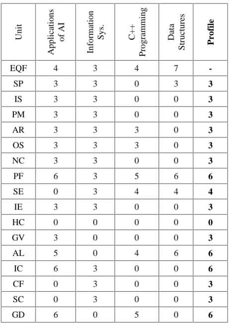
A system for profiling educators was required once all units of study were given measures of understanding within the taxonomy. Initial educator profiles were derived by algorithmically finding the highest measure of understanding delivered by that educator (illustrated in Table 6).
Table 6. An example of an educator’s derived profile.
U
n
it
A
p
p
li
ca
ti
o
n
s
o
f
A
I
In
fo
rm
at
io
n
S
y
s.
C+
+
P
ro
g
ra
m
m
in
g
D
at
a
S
tru
ct
u
re
s
P
ro
fi
le
EQF 4 3 4 7
-SP 3 3 0 3 3
IS 3 3 0 0 3
PM 3 3 0 0 3
AR 3 3 3 0 3
OS 3 3 3 0 3
NC 3 3 0 0 3
PF 6 3 5 6 6
SE 0 3 4 4 4
IE 3 3 0 0 3
HC 0 0 0 0 0
GV 3 0 0 0 3
AL 5 0 4 6 6
IC 6 3 0 0 6
CF 0 3 0 0 3
SC 0 3 0 0 3
GD 6 0 5 0 6
However, this in itself is insufficient for purposes as it limits educators to profiles that cover their existing assignments, which may not adequately express their expertise or areas that they may want to grow into with suitable staff development. All staff specified all units of study that they would, could and could not deliver.
This approach allowed for the addition of units that each educator could deliver to those currently delivered and the production of a tabled populated with meaningful measures against each knowledge area along with a specified target number of units for assignment to that educator. Here, pro rata to their contracted teaching responsibility, lecturers receive five units, principal lecturers/readers receive four units and others receive three units.
Profiling educators in terms of units of study provides boundaries within which educators can be moved. For example, educators with strong IT profiles will tend towards being allocated to units of study within the IT subject area. Algorithmically determining a list of educators with the minimum profile required for delivering each unit of study is both useful in terms of informing the search process documented here and in terms of highlighting where unit delivery is at risk due to a lack of knowledge area expertise within the staff pool. Allocating educators that closely match required knowledge retains expertise within the deployment pool for later assignment with the result that strong generalists tend to be allocated last, being defined as highly regarded
‘sweepers’ by management.
[image:3.595.51.266.188.523.2]target assignment of zero units directs search towards early solutions that minimizes assignments against ‘Other, A.N.’
with further manipulation following. The next section provides further detail on generation of solutions.
4. GENETIC ALGORITHM SOLUTION
Given the scale of the problem and its solution by heuristic processes applied by management introduced to the reader in the previous sections, this section provides an overview of a genetic algorithm and the solution methodology adopted. Genetic algorithms [2, 3] are adaptive search methods used to solve optimisation problems. They mimic the genetic process of evolution within biological organisms by means of natural selection and adaption.A GA is able to ‘evolve’ solutions toreal worlds by mimicking this process [4]. Its widespread use evidences both the adaptability and efficiency of the approach, with it having been successfully applied to obtain optimal and near optimal solutions to such problems as scheduling [5], timetabling [6], frequency assignment [7], attribute selection [8] and layout optimisation [9].
Solutions are evolved by means of a genome (or structure of the problem, where a single instance represents a solution to the problem) and a genetic algorithm (the procedure utilised to control how evolution takes place). The GA makes use of operators applied to the genome and selection/replacement strategies controlled by the genetic algorithm that generate new, ideally better, individuals. The GA utilises an objective function to determine how fit each of the genomes is for survival. Given a choice of GA, the following outlines three components required to solve a problem:
The structure of the problem must be defined and a representation for the genome determined;
Given the genome, define suitable generic operators; Using the genome, define an objective function that
measures the relative quality of a solution.
In summary, when using a GA to solve an optimisation problem, a combination of a series of variables within a genome provides a single solution to the problem. The GA creates a population of genomes from which to select parents for reproduction and evolution through the application of selection, crossover and mutation. Here, fitter parents tend to be selected more often for recombination utilising a crossover operator where elements from each parent are put together to create offspring. The tendency for selection of fitter parents intensifies search around more promising areas. The application of a mutation operator on small parts of an offspring has the effect of diversifying the search into other areas by promoting genetic diversity within the population. The GA operates on each generation of the population to evolve an optimum, or near optimum, solution to the problem measured by the objective function. The following sections expand on each of these components.
4.1 The Genome
A good data structure for a genome is both minimal and completely representative. For example, if a real value and a number of integers can represent a solution to a problem, then the definition of the genome’s data structure utilises these characteristics. The representation should not include any information other than what is required to express a solution to the problem. Additional data structures called alleles provide ranges of acceptable values for each constituent part of the genome. Here, each element of the genome, or gene, maps to an individual unit populated by an integer taken from
predetermined and separate pools of educators with the appropriate background for delivery. Finally, each genome has a ‘fitness’ score associated with it that determines its prospects for selection.
4.2 The Genome Operators
Initialisation, mutation and crossover operators allow for a particular population bias, recombination of parents and mutations specific to the problem representation. An
initialisation operator ‘filled’ each gene with a randomly selected member of its corresponding allele to provide ninety percent of a starting population of diverse allocations from which to evolve a final solution. The genomes making up the remainder of the population map to the allocation rolled forward from the previous academic year to help minimise disruption to existing allocations, which are inherently sensible and useful for determining future assignments.
The crossover operator defines the procedure for generating a child from two parent genomes. The crossover operator
produces new individuals as ‘offspring’, which share some features taken from each ‘parent’. Here, two-point crossover is utilised, which is to say that a set of genes with random start and end points taken from within the genome are crossed over between parents to form two offspring.
Finally, the mutation operator defines the procedure for mutating the genome. Mutation, when applied to a child, randomly alters a gene with a small probability. This provides a mechanism for (re)introducing genetic diversity into the population and helps prevent convergence around a local optimum. Here, the mutation operator replaces a gene with a randomly selected member of its allele set.
4.3 Objective Function and Scaling
The success of any optimisation problem rests upon its objective function, the purpose of which is to measure relative solution quality. The objective function used here works by calculating and summing the costs associated with the assignment of educators to units of study within the state representation.
The quality of a given configuration is an abstraction of the fitness of individuals to deliver units of study, balanced workload, minimising change to established assignments and ensuring mixed delivery teams in cases where a programme of study encompasses 10 ECTS credits. Suitable candidates for delivery of each unit are determined prior to commencing the search process so as to identify the neighbourhood of a given solution quickly at run-time.
4.3.1 Solution Evaluation
The objective function used to evaluate teaching assignment solutions requires a number of definitions that model the
problem’s underlying structure, specifically:
EOi= 90 if unit i is part of a larger module delivered by the same educator else 0;
COij= 1 if the educator j assigned to a unit i differs from the original else 0;
SOi= the sum of skills assigned to a unit i above that necessary for delivery;
LOij= 1 if educator j is assigned to unit i else 0;
Αis a 2D matrix of educator under and over assignment scaling factors;
LEjis the target number of assignments for educator j; n is the number of units of study;
p is the number of educators;
4.3.2 Objective Function
The objective function examines the weighted relationship of assignments. The general expression of the objective function is shown in (1). Here fi and wi represent, respectively, a function that measures an aspect of the overall quality of a solution and the weight of that particular measure, with a low value of f0(s) indicating a good solution.
(1)
The first term f1given in (2) penalises a solution where the same educator delivers multiple units that are part of the same programme of study (module). This is a management priority given the typically large size of modules (10 ECTS credits).
(2)
The second term f2given in (3) counts the changes made to
each educator’s assignment and sums a scaled product of each
count. Here, minimising the number of changes made to an
educator’s assignment will minimise stress, with large
changes incurring broadly geometric increases in cost.
(3)
The matrix Γ is given in (4) below.
Γ = 0 8 16 32 64 128 256 512 1024 2048 4096 (4)
The third term f3 given in (5) sums the over-skilling of educator to unit assignments. Here, minimising excess skill assignments to units retains expertise within the educator pool for assignment elsewhere.
(5)
The last term f4given in (6) counts the number of assignments given to an educator and sums a scaled product of each count that is proportional to the maximum number of assignments that a given educator can be given. Here, under or over-assignment will be penalised, with larger values incurring broadly geometric increases in cost.
(6)
Here, the two-dimensional matrix Α is populated with costs
that are proportionate to the target number of assignments, which range from 0 to 5. Costs are punitive for all rows beyond column 10, with only the first row (associated with
‘Other, A.N.’) having values that are used in practice.
Penalties for over-assignment are higher, for example, for a reader or a part-time educator than for a lecturer. The matrix values for the first ten columns of each row of the matrix are shown in (7), with further extrapolation being an easy matter.
Α =
0 256 512 1024 2048 2100 2200 2300 2400 2500 2600
(7)
0 128 256 512 1024 2048 2100 2200 2300 2400 2500 0 64 128 256 512 1024 2048 2100 2200 2300 2400 0 32 64 128 256 512 1024 2048 2100 2200 2300 0 16 32 64 128 256 512 1024 2048 2100 2200 0 8 16 32 64 128 256 512 1024 2048 2100
Genetic algorithms are often more attractive than gradient search methods because they do not require complicated differential equations or a smooth search space. The genetic algorithm needs only a relative measure of genome fitness. The objective function provides this, needing only a genome, or solution, and genome specific instructions for assigning and returning a measure of the solution's quality. The objective score is the raw value returned by the objective function. The fitness score is the possibly transformed objective score used by the genetic algorithm to determine the fitness of individuals for mating.
n
o
o
f
n
j j
i i
0
(8)
Sigma Truncation [4] incorporates problem dependent information into the mapping. Here, (8) transforms objective scores (o) into fitness values (f) utilised for selection, where n is the population size andis its standard deviation.
4.4 The Genetic Algorithm
The Genetic Algorithm initialises the population, determines which individuals should survive, which should reproduce and which should die. At each generation, individuals selected as candidates for parenthood combine elements from each parent to produce offspring. Offspring may then undergo mutation. Insertion of offspring into a population together forms the set of potential parents for the next generation. Evolution terminates upon meeting a given condition, such as a fixed number of generations, fitness of the best solution, population convergence, or any problem specific criterion.
Of the variations of GA, the work presented in this paper utilised a derivation of the Steady State GA [10]. This GA uses overlapping populations with a pre-specified amount of overlap (expressed here as a percentage). At each generation, the GA creates a temporary population of new individuals utilising roulette wheel selection [4], adds these to the previous population and then removes weaker individuals sufficient to return the population to its original size. Evolution ends when the bestindividual’s fitnessdivided by the population mean is greater than the desired ratio, at which point population diversity is such that further generations amount to little more than a random walk.
5. COMPUTATIONAL EXPERIMENTS
The genetic algorithm, implemented in C++ under Windows 7, ran on an AMD Bulldozer FX-8 (8x3.1 GHz) with 8 MegaBytes of RAM. Experiments utilised a dataset with 167 deliverable units spanning levels 3 through 7 and 45 educators. Algorithm parameters for the results presented in this paper were determined empirically and set as follows: w1, 9000.0; w2, 20.0; w3, 2.0; w4, 4.0; mutation, 0.03; population size, 250; population overlap, 0.1; and ratio, 0.95.f
0( )
s
=
(
f
1×
w
1)
+
(
f
2×
w
2)
+
(
f
3×
w
3)
+
(
f
4×
w
4)
f1
=
EO
ii=0
n
∑
f2
= Γ
CO
iji i=0n
∑
j=0
p
∑
f3
=
SO
i i=0n
∑
f
4= Α
LO
ij−
LE
ii n
∑
j=0
m
Fig. 1 presents the fitness of the best individual at 10-generation increments. Here, the cost of the first 50 generated solutions falls rapidly as unassigned units are distributed and existing assignments adjusted to accommodate the new units. As the algorithm is first encouraged to make these assignments, scores are disproportionately large until only a few of these assignments remain. Consequently, the graph does not show early generation fitness scores.
Fig 1: Generational Fitness Scores.
Here, evolution continues for 5300 generations, meaning that the algorithm evaluates upwards of 182000 solutions. Un-optimised execution time amounts to minutes.
The solution makes 34 new assignments across 20 educators, with 2 new units allocated to 3 educators and more than 2 allocated to one new member of staff, and with 19 existing allocations moved. Lack of provision in some areas resulted in outsourcing to colleagues within Law, Business and Science.
6. CONCLUSION
The method resulted in an applicable solution to a problem where a combination of voluntary severance, retirement, replacement and additional units of study required the assignment of 18 vacant units while minimising disruption to existing staff assignments. The solution formed the plan for the coming academic year, but within a small fraction of management time normally attributed. The solution highlighted skill shortages and informed strategies for filling these gaps. The plan elicited approximately one sixth of the change requests delivered in the previous year.
The approach translated well to the development of heuristically determined solutions to the teaching assignment problem, specifically that:
The GA’s intensification and diversification strategies allowed for an effective search of the problem space before ultimately converging around a good solution;
Sensitivity to the starting point by the introduction of a number of starting points into the population that had been derived from the previous year’s allocationhelped mitigate against overly different solutions and the overheads of varying educator workloads;
The definition of good allele structures is particularly helpful in this context given the profiled relationships between educators and units;
The problem itself does not require continuous optimisation, i.e. the periodically generated solutions can be adapted through the manipulation of parameters.
The process has informed management decision making for continuity planning, facilitated scheduling for the coming academic year and informed the process of staff acquisition from other areas where local expertise was insufficient for needs. Although the provision of specific results is problematic given the volume of data and the confidential nature of educator profiles, this paper has described the process by which teaching assignment solutions are determined in sufficient detail for replication within other computer science departments.
7. REFERENCES
[1] The Joint Taskforce for Computing Curricula 2005. Computing Curricula 2005. ACM & IEEE., ISBN: 1-59593-359-X.
[2] Holland, J. H. 1975. Adaption in Natural and Artificial Systems. University of Michigan Press, Ann Arbor.
[3] Turing, A. P. 1948. Intelligent Machinery in: Cybernetics: Key Papers 1968. eds Evans, C. R. and Robertson A.D.J., University Park Press.
[4] Golberg, D. E. 1989. Genetic Algorithms in search, optimization and machine learning. Addison-Wesley.
[5] Hou, E.S.H, Ansari, N. and Ren, H. 1994. A genetic algorithm for multiprocessor scheduling. Parallel and Distributed Systems, IEEE Transactions on, 5(2), 113-120.
[6] Aickelin, U. and Dowsland, K.A. 2004. An indirect genetic algorithm for a nurse-scheduling problem. Computers & Operations Research, 31(5), 761-778.
[7] Valenzuela, C, Hurley, S. and Smith, D. 1998. A permutation based genetic algorithm for minimum span frequency assignment. In: Parallel Problem Solving from Nature-PPSN V, Springer Berlin Heidelberg, 907-916.
[8] Wilson, I.D., Jones, A.J., Jenkins, D.H. and Ware, J.A., 2005.Predicting housing value: genetic algorithm attribute selection and dependence modelling utilising the Gamma Test. Adv. in Econometrics 19, 243-275.
[9] Wilson, I.D., Ware, J.M. and Ware J.A., 2003. A genetic algorithm approach to cartographic map generalization. Computers in Industry 52(3), 291-304.
[image:6.595.54.278.162.308.2]