Attribute Level Clustering Approach to Quantitative Association Rule Mining

Attribute Level Clustering Approach to Quantitative

Association Rule Mining

M.Phani Krishna Kishore

Gayatri Vidya Parishad College of Engineering(Autonomous)

Visakhapatnam,AP, India

Ashok Kumar Madamsetti

Gayatri Vidya Parishad College of Engineering(Autonomous)

Visakhapatnam,AP, India

ABSTRACT

Generating rules from quantitative data has been widely studied ever since Agarwal and Srikanth explored the problem through their works on association rule mining. Discretization of the ranges of the attributes has been one of the challenging tasks in quantitative association rule mining that guides the rules generated. Also several algorithms are being proposed for fast identification of frequent item sets from large data sets.

In this paper a new data driven partitioning algorithm has been proposed to discretize the ranges of the attributes. Also a new approach has been presented to create meta data for the given data set from which frequent item sets can be generated quickly for any given support counts.

General Terms

Information systems, Data mining,Information systems, Association rules

Keywords

Quantitative association rule mining, association rule mining.

1.

INTRODUCTION

Association rule mining has become one of the prime research area which attracted the attention of the researchers from diverse fields. With the advent of the business intelligence concepts it gained commercial edge as well. Ever since [Agarwal et al. 1994] [Agarwal et al. 1996] posed the problem numerous researchers proposed variations, advancements and enhancements to the process.

As a special case, generating quantitative association rules from the data containing transactions with attributes containing numeric and categorical values as well has emerged. To introduce the notation, and to be consistent with the existing literature, Let U = ( D, A ) denote an information system or data table, where D = { T1,T2,…,Tn } denote the set of transactions, A = { a1, a2 ,a3, … , an} denote the set of all attributes which may contain both numeric as well as categorical values. Each attribute may take a value in a prescribed range of values [ Vi, Vi



]. i.e., Tj ( ai ) = Vij, where Vij  [Vi , Vi ]. A quantitative association rule is an implication of the form X  Y, where X, Y are strings of attributes of the form , ], ,

, ] , ], , , The problem is to find suitable and meaningful attributes and their ranges.

To find such rules several researchers proposed various methods. [14] Agarwal et al., proposed partitioned the ranges into equi-depth bins. Then they applied apriori algorithm to find the frequent item sets. The approach works if all the values of attribute are equally distributed. [12 ] Brian Lent et al. combined similar association rules to form interesting

quantitative association rules using the technique of clustering. The algorithm will map the whole database into a two-dimensional array with each entry representing an interval in each of the dimensions. [9 ] Wang Lian et al. used the technique of identifying dense regions in the hyper-rectangular space and there by identifying the quantitative association rules. This method works if the data is spread in pockets. Also this method clusters the data at transactions level. Recently [1 ] Vincent S. Tseng et al. proposed a utility based algorithm that produces less number of item sets and which are more relevant. [3 ] Shih-Sheng Chen et al. proposed model that can handle multiple supports to produce more precise quantitative association rules. [11] Qiang Tong et al., proposed a mechanism in which rules are generated on overlapped intervals.

[

16

]

Huizhen Liu, et al., viewed the data table as a matrix and devised methods to find quantitative association rules using matrix operations. [17] Shuhong Zhang et al., in their work had proposed mechanisms to derive fuzzy quantitative association rules. [6] Lenca, P, gave a detailed analysis on the interestingness measures for association rules. [7] Nitin Gupta, et al applied the concepts of evolutionary computation techniques in the form of genetic algorithm is used to find quantitative association rule mining to protein sequences.

1.1

Motivation for the present work

In case of large data with numerical or categorical attributes in real time data sets, each attribute may have its own characteristic variations depending on the nature of the data. Hence it seems natural to cluster the attribute values independently and identify the inherent nature of the distribution of the attribute values, instead of cluster the data at transaction level. Also for identifying frequent item sets a vast collection of algorithms that suit different data types with better performance is also available in literature. However these algorithms need to operate for each set of parameters being chosen. In this direction a new way of creating Meta data is proposed which helps to identify the frequent item sets quickly without going into the actual data sets.

2.

PROPOSED CLUSTERING

ALGORITHM

The goal of any clustering algorithm lies in finding clusters in which similar (with respect to specified distance measure) items are grouped into one cluster. Usually similar items are nearer to each other when compared to outliers. Outliers lie far away from the regular data points. Based on the spread of the values in the n-dimensional space in this section an algorithm is proposed that groups the data items.

ALGORITHM 1. Clustering algorithm:

__________________________________________________ Input: Data set

Output: clusters C1,C2,…,Cm Let D = {a1, a2,…, an} be a data set.

Step 1 : compute inter point distance for each pair ( ai, aj ) where 1≤i ≤ n and 1 ≤ j ≤ n.

Step 2 : compute nearest neighborhood distance di for each ai.

Step 3 : Let (d1,n1), (d2,n2), (d3,n3), ..., (dk, nk) be nearest neighbor distances, frequency of

occurrences.

Step 4 : Compute α to be the distance at which 

    _*d

100 N

of the data items possess

nearest neighbors, where N= Number of Transactions, d = percentage of data items to be considered. Step 5 : Initialize cluster C1 with a1

Step 6 : Compute distance d(a1,a2) if d(a1,a2) ≤ α

C1={a1,a2} else

set C1={a1}, C2={a2} Step 7 : Compute d(a1,a3)

if d(a1,a3) ≤ α then C1 = C1 {a3} else

compute d(a2,a3).

If d(a2,a3) ≤ α then C2 = C2 {a3} else

Initialize C3 = {a3}.

Step 8 : Continue this process for all data items.

At the end of the process let C1, C2, C3,…, Cl be the clusters formed.

/*Cluster Merging */

Step 9 : For each data item in C2, compute distance with each item of C1.

Step 10 : If distance is less than or equal to α for at least one item then

merge C1, C2 and set C1 = C1 C2. Update C1,C2,…Cl as C1,C2,…C l-1 Otherwise

Repeat the above process for C2 with other clusters Step 11 : Repeat steps 9,10 until no further merging is possible.

__________________________________________________ At the end of the above process final cluster will be identified. In the above algorithm α is the only parameter that determines the nature and size of the clusters.

This algorithm identifies the inherent clusters in the sense that only outliers will remain distant from the remaining points and α determines the level of separation. Usually the value of

α against the number of clusters formed gets stabilized at certain level and hence α is not a sensitive parameter. The detailed analysis is shown in section 4.

3.

NEW APPROACH TO FIND

FREQUENT ITEM SETS

In this section a novel approach is presented to find the frequent item sets using apriori property.

3.1

Graph representation

Given a Boolean data table construct a edge labeled graph (T, A) with transactions as vertices. Given a pair of vertices (Ti, Tj) add an edge if the corresponding cell entry in the newly constructed data table is 1. Add the string of attributes that are common to the pair of transactions Ti, Tj in the newly constructed table as a label for the edge between Ti, Tj. This produces an undirected graph with edge labels.

The meta data matrix corresponding to the above graph is an upper triangular matrix with cell entries as the labels. The presence of an attribute in a cell indicates that the attribute is present in two transactions. Thus support count for each entry is of minimum 2. From this meta data table the support count of each attribute can be calculated directly without going into the original data table.

Let a set of attributes Ai be present in a cell corresponding to Ti, Tj . Now if Ai is also present in another cell (as complete or as a subset) corresponding to Ti, Tk then support count of Ai is increased by 1. If it is present in cell corresponding to Tr, Tk then increase the support count by 2 . By using this process the support count for all possible sets of attributes can be calculated without visiting the actual data set.

From the meta data given a minimum support count, the frequent item sets can be found by repeatedly locating the cell with highest number of entries satisfying the minimum support count until all the attributes are covered.

The advantage of this method when compared with the apriori algorithm lies in the fact that the original data table is read only once to create the meta data table. Once the table is created the original table can be discarded and for any given support count the frequent item sets can be easily found from the meta data which makes the process quicker. A detailed performance evaluation is done in section 4 . This algorithm is compared with apriori algorithm for its performance and observed better results.

3.2

Quantitative association rule mining

algorithm

In this section a new quantitative association rule mining algorithm is proposed.

corresponding to ranges, which creates a new data table in which transactions remains same as that of the original table but with increased number of attributes. Each cell of the newly constructed table consists of either 0 or 1 in accordance with the corresponding attribute value for the given transaction falls in the range prescribed or not. The newly constructed data table is a Boolean data table.

Now construct a meta data table that contain information of 2-frequent item sets for the Boolean data table. Now given a minimum support count the most frequent item sets can be calculated from the meta data.

Generate the rules corresponding to the frequent item sets. Since the attributes in the meta data table corresponds to different ranges of the original attributes, from the rules generated as given above the quantitative association rules can be described.

ALGORITHM 2. Quantitative Association Rule Mining Algorithm

__________________________________________________ Input: Data table D (A1,A2,…,An) with numeric and/or categorical attribute values.

Output: Quantitative association rules

Step1: For each attribute Ai (1 ≤ i ≤ n) identify the clusters by using the clustering method as specified in section -1.

Step-2: Identify the minimum and maximum for each cluster of each attribute and create new attributes by subdividing the original attributes accordingly. Step-3: Form a Boolean matrix B = [bij] with transactions and newly created attributes with bij = 1 if transaction Ti contains the value in the range of newly created jth attribute; 0 otherwise.

Step4: Construct a meta data table as specified in section 2 and identify the support counts.

Step5: For a given minimum support count identify the frequent item sets from the meta data table constructed as above and form the quantitative association rules.

____________________________________________

3.

Example:

The above process is illustrated using an example. Consider the data table consisting of 5 attributes with 3 of them as numeric and 2 of them as categorical and 10 transactions.

Table:1 sample data set

I1 I2 I3 I4 I5 I6 I7 I8 I9 I10 I1 0 9 4 19 18 44 35 18 17 4 I2 9 0 5 10 9 35 26 9 8 5 I3 4 5 0 15 14 40 31 14 13 0 I4 19 10 15 0 1 25 16 1 2 15 I5 18 9 14 1 0 26 17 0 1 14 I6 44 35 40 25 26 0 9 26 27 40 I7 35 26 31 16 17 9 0 17 18 31 I8 18 9 14 1 0 26 17 0 1 14 I9 17 8 13 2 1 27 18 1 0 13 I10 4 5 0 15 14 40 31 14 13 0

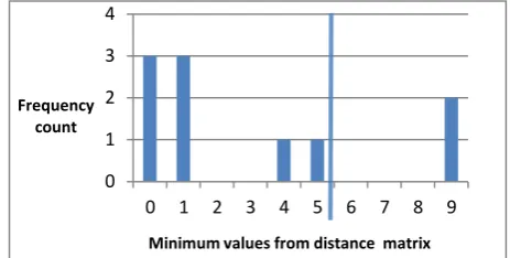
[image:3.595.316.548.73.190.2]

Min 4 5 0 1 0 9 9 1 1 0

Fig 1.Frequency distribution of nearest neighbor distances

The frequency diagram and the cutoff value d = 80%. The value of α = 5

Clusters of Attribute A1 after the first step are

c1= {23, 27, 27}, c2= {32}, c3= {42,41,41,40}, c4= {67}, c5= {58}

After merging the related clusters

c1= {23,27,27,32}, c2= {42,41,41,40}, c3= {67}, c4= {58} Consider interval of each cluster as the new attribute (Split of a original attribute).

A11= [23-32] A12= [40-42] A13= [67] A14= [58]

Similarly the other attributes A2, A3 are also clustered using d = 90 and the new attributes after splitting is obtained as, Clusters of Attribute A2:

c1= {0.8,0.8,0.9}, c2= {0.6},c3= {0.2,0.3,0.4,0.2,0.3,0.4}, Take each cluster as one interval

A21= [0.2 - 0.4] A22= [0.6] A23= [0.8 - 0.9] Clusters of Attribute A3

c1= {101,103,107,111,106,104,103}, c2={121}, c3= {128,129}

Take each cluster as one interval

[image:3.595.320.550.552.680.2]

A31= [101-111], A32= [121], A33= [128-129] Table 2: Nearest neighbor distances

Attributes A4 and A5 are categorical. So the class labels can be considers as clusters. Attribute A4 contains three class labels, so the number of clusters are 3. Attribute A5 contains two class labels, so the number of clusters are 2.

A41= {High} A42= {Medium} A43= {Low}, A51= {M} A52= {F}

TId A1 A2 A3 A4 A5

I1 23 0.8 101 High Yes

I2 32 0.6 103 Medium Yes

I3 27 0.8 107 Medium No

I4 42 0.9 121 High No

I5 41 0.2 128 Low No

I6 67 0.3 129 Low Yes

I7 58 0.4 111 Low No

I8 41 0.2 106 Medium No

I9 40 0.3 104 High Yes

I10 27 0.4 103 High Yes

0 1 2 3 4

0 1 2 3 4 5 6 7 8 9

Frequency count

Boolean Matrix: As described in step3 the new data table is created in the form of a Boolean matrix corresponding to the new attributes.

Table3. Boolean matrix

Record Id

A1 A2 A3 A4 A5

A11 A12 A13 A14 A21 A22 A23 A31 A32 A33 A41 A42 A43 A51 A52

I1 1 0 0 0 0 0 1 1 0 0 1 0 0 1 0

I2 1 0 0 0 0 1 0 1 0 0 0 1 0 1 0

I3 1 0 0 0 0 0 1 1 0 0 0 1 0 0 1

I4 0 1 0 0 0 0 1 0 1 0 1 0 0 0 1

I5 0 1 0 0 1 0 0 0 0 1 0 0 1 0 1

I6 0 0 1 0 1 0 0 0 0 1 0 0 1 1 0

I7 0 0 0 1 1 0 0 1 0 0 0 0 1 0 1

I8 0 1 0 0 1 0 0 1 0 0 0 1 0 0 1

I9 0 1 0 0 1 0 0 1 0 0 1 0 0 1 0

I10 1 0 0 0 1 0 0 1 0 0 1 0 0 1 0

The graph that represents the above data table and the corresponding Meta data table is given by

Fig:2.Graph of transactions

Table:4. Metadata table

T 1

T 2

T 3

T 4

T 5

T 6

T 7

T 8

T 9

T1 0

T1 0

a, h, n

a, g, h

g, k

N U LL

n h h

h, k, n

a,h, k,n

T2 0

a, h, l

N U LL

N U LL

n h h,_l h,_n a,h,_n

T3 0 g,_o o

N U LL

h, o

h, l, o

h a,h

T4 0 b,_o

N U LL

o b,_o b,_k k

T5 0

e, j, m

e, m ,o

b, e, o

b,

e e

T6 0 e,_m e e,_n e,n

T7 0

e, h, o

e,

h e,h

T8 0

b, e, h

e,h

T9 0 e,h,_k,n

T1

0 0

Where A11= a , A12= b, A13= c A14= d, A21= e, A22= f A23= g , A31= h, A32= I, A33= j, A41= k, A42= l, A43= m, A51= n , A52= o .

From the above table, the frequent item sets of support count 2 are { a,h,k,n } and {e,h,k,n} because these are the maximum number of intervals which satisfies the minimum support count 2.

In the similar manner, the frequent item sets of support count 3 are { a,h,n } and {h,k,n} because these are the maximum number of intervals which satisfies the minimum support count 3.

The rules generated for the 3-frequent item set { a,h,n }are as follows :

Rules generated with Min.sup =3 and Min.conf =100%

(α) Cut off: 70%

C ( 103.0 - 104.0 ) => E ( Yes )

(α) Cut off 80%

A ( 23.0 - 32.0 ) ^ E ( Yes ) ^ => C ( 101.0 - 107.0 )

C ( 101.0 - 107.0 ) ^ D ( High ) ^ => E ( Yes ) D ( High ) ^ E ( Yes ) ^ => C ( 101.0 - 107.0 )

(α) Cut off 90%

C ( 101.0 - 111.0 ) ^ D ( High ) ^ => A ( 23.0 - 42.0 ) ^ E ( Yes )

A ( 23.0 - 42.0 ) ^ C ( 101.0 - 111.0 ) ^ D ( High ) ^ => E ( Yes )

D ( High ) ^ E ( Yes ) ^ => A ( 23.0 - 42.0 ) ^ C ( 101.0 - 111.0 )

A ( 23.0 - 42.0 ) ^ D ( High ) ^ E ( Yes ) ^ => C ( 101.0 - 111.0 )

4.

EXPERIMENTAL RESULTS

The algorithm is tested on a bench mark data set taken from the UCI Machine learning repository. (http: //archive .ics .uci . edu / ml / datasets /Abalone).The data is restricted to 1000 data items. The purpose of the data is to Predict the age of abalone from physical measurements. The age of abalone is determined by cutting the shell through the cone, staining it, and counting the number of rings through a microscope -- a boring and time-consuming task.

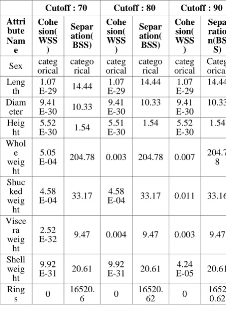
Since clustering task is involved the validity of the clusters is measured through Cohesion and Separation. The following table illustrates the values obtained at different cutoff levels (α) for all the attributes.

[image:5.595.54.277.277.583.2]

It is observed that the cohesion values in each case are very small when compared with the corresponding separation values which indicate a fairly reasonable clustering.

Table.5. Cluster validation

Cutoff : 70 Cutoff : 80 Cutoff : 90 Attri bute Nam e Cohe sion( WSS ) Separ ation( BSS) Cohe sion( WSS ) Separ ation( BSS) Cohe sion( WSS ) Sepa ratio n(BS S)

Sex categ orical catego rical categ orical catego rical categ orical Categ orical Leng th 1.07

E-29 14.44 1.07 E-29

14.44 1.07 E-29

14.44 Diam

eter 9.41

E-30 10.33 9.41 E-30

10.33 9.41 E-30

10.33 Heig

ht

5.52

E-30 1.54 5.51 E-30

1.54 5.52 E-30 1.54 Whol e weig ht 5.05

E-04 204.78 0.003 204.78 0.007 204.7 8 Shuc ked weig ht 4.58

E-04 33.17 4.58

E-04 33.17 0.011 33.16 Visce

ra weig

ht

2.52

E-32 9.47 0.004 9.47 0.003 9.47 Shell

weig ht

9.92

E-31 20.61 9.92

E-31 20.61 4.24

E-05 20.61 Ring

s 0

16520.

6 0

16520.

62 0

1652 0.62 The performance of the new algorithm is compared in two ways. In the first phase the time (in sec.) for finding association rules from the Boolean matrix(after discretization) is compared with apriori algorithm. It is observed that the proposed method is performing well compared to the apriori method.

In the second phase the rules obtained by the proposed algorithm are compared with that of the rules obtained in equi-width binning method. Less number of rules are observed.

The proposed method can be made more scalable by employing advanced methods of dealing with sparse matrices. The following are the results obtained.

Table6. Performance Comparison

Support

Count 2 3 4 5

Tim e in S ec o n d s No. of Data Point s Ap rio ri Pro pos ed Met hod Ap rio ri Pro pos ed Met hod Ap rio ri Pro pos ed Met hod Ap rio ri Pro pos ed Met hod

100 1.9 7

3.06 2

0.6 6 4.52

0.3 8 4.69

0.2 9 3.59 200 8.2₈ 4.44 2.8₁ 4.43₇ 1.4₅₃ 4.11 0.7₀ 3.83 300 20.₄₈ 4.86 8.2₈ 5.23₄ 4.3₂₉ 4.20₃ 2.2₅ 4.03 500 63.₉₂ 7.02 32.₀₈ 5.78₁ 18 7.73₅ 10.₂₅ 8.29 700 8.115

5 10.1

3 77.64 15.20 35.86 11.625 29.09 9.95 900 7.631

7 15.0 5 12 8.8 6 17.5

93 61.47 12.80 51.95 16.37 1000 3.438

0 20.5

9 16 6.7

8 20 10 6.3 1

18.7

3 66.17 21.45

In graphical form

0 50 100 150 200 250 300 350 400 450 Time in Seconds

Number of Transactions

Apriori

QARM

Support count -2

0 20 40 60 80 100 120 140 160 180 Time in Seconds

Number of Transactions

Apriori

QARM

The rules are also generated on the data with various combinations of input parameters.

*Rules generated with min. support =5 and min. confidence=100% and (α) cut off 90%

1. SEX ( Infant ) ^ DIAMETER ( 0.25 ) ^ WHOLE WEIGHT ( 0.1655 - 0.1835 ) =>VISCERA WEIGHT (0.0335 - 0.051)

2. SEX (Infant ) ^ SHUCKED WEIGHT ( 0.0065 - 0.008 ) =>

WHOLE WEIGHT (0.013 - 0.024) ^ VISCERA WEIGHT ( 0.002 - 0.0065 )

3. SEX (Infant ) ^ WHOLE WEIGHT ( 0.013 - 0.024 ) ^ SHUCKED WEIGHT ( 0.0065 - 0.008 ) => VISCERA WEIGHT (0.002 - 0.0065)

4. SEX (Infant ) ^ SHUCKED WEIGHT ( 0.0065 - 0.008 ) ^ VISCERA WEIGHT ( 0.002 - 0.0065 ) => WHOLE WEIGHT (0.013 - 0.024)

5. SEX (Infant ) ^ SHELL WEIGHT ( 0.005 ) => WHOLE WEIGHT (0.013 - 0.024) ^ VISCERA WEIGHT ( 0.002 - 0.0065 )

6. SEX (Infant) ^ WHOLE WEIGHT ( 0.013 - 0.024 ) ^

SHELL WEIGHT ( 0.005 ) => VISCERA WEIGHT (0.002 - 0.0065)

7. SEX (Infant ) ^ VISCERA WEIGHT ( 0.002 - 0.0065 ) ^

SHELL WEIGHT ( 0.005 ) => WHOLE WEIGHT (0.013 - 0.024)

8. SHUCKED WEIGHT ( 0.0065 - 0.008 ) ^ SHELL WEIGHT ( 0.005 ) =>

WHOLE WEIGHT (0.013 - 0.024) ^ VISCERAWEIGHT ( 0.002 - 0.0065 )

9. WHOLE WEIGHT ( 0.013 - 0.024 ) ^ SHUCKED WEIGHT ( 0.0065 - 0.008 ) ^ SHELL WEIGHT ( 0.005 ) => VISCERA WEIGHT ( 0.002 - 0.0065 )

10. SHUCKED WEIGHT ( 0.0065 - 0.008 ) ^ VISCERA WEIGHT ( 0.002 - 0.0065 ) ^ SHELL WEIGHT ( 0.005 ) => WHOLE WEIGHT ( 0.013 - 0.024 )

A detailed analysis is made on how the rules are being generated for different values of alpha(α) and for different equiwidth intervals.

The following table illustrates the number of rules generated in the proposed method in comparison with the equi-width method.

Table.7. Rules comparison

Min. Confidence : 100%

Number of rules for each cutoff percentage

Number of rules in trials with different equi-width

divisions Support 70% 80% 90% 95% I II III

2 157 148 427 242 910 999 178 3 104 14 70 86 619 606 147

4 13 4 8 85 479 481 132

5 1 1 10* 27 405 419 132

20 0 0 0 0 111 177 95

30 0 0 0 0 64 123 82

40 0 0 0 0 52 28 74

In quantitative association rule mining several methods are being proposed by researchers. Equi-width and Equi-depth binning are the two most prominent methods of identifying the ranges of the attributes. Both the methods suffer from the drawbacks. In equi-width binning method unless prior knowledge of the ranges of attribute values is available the division is by no means reasonable and the rules generated are highly sensitive to the division. Where as in equi-depth binning the prior knowledge of the frequency plays the role. In the proposed method if the data is not uniformly spaced and if clusters are well separated then more meaningful and stable rules can be generated so that two tasks of identifying the underlying clusters and rules among the clusters can be identified.

Another advantage of the proposed method is that any well performing clustering method can be embedded into the process like DBSCAN, K-MEANS etc., as per the user requirement.

4.1

Conclusion

In this work a quantitative association rule mining algorithm is proposed using a discretization procedure which forms the inherent clusters for discretizing the quantitative attributes. A procedure for creating metadata which can be used to generate frequent item sets for a given support count, without going into actual dataset again is presented and observed that this processes fastens the computation of frequent item sets over the apriori algorithm.

From the experimental results, it is observed that in the proposed method discretization procedure is more effective

0 20 40 60 80 100 120

Time in Seconds

Number of Transactions

Apriori

QARM

Support count -4

0 10 20 30 40 50 60 70

Time in Seconds

Number of Transactions

Apriori

QARM

behavior of attribute values and tries to capture the group behavior in terms of association rules.

5.

REFERENCES

[1] Vincent S. Tseng, Bai-En Shie, Cheng-Wei Wu, and Philip S. Yu, “Efficient Algorithms for Mining High Utility Item sets from Transactional Databases” ,IEEE transactions on knowledge and data engineering, vol. 25, no. 8, august 2013.

[2] Ansaf Salleb-Aouissi, Christel Vrain, Cyril Nortet ,Xiangrong Kong Vivek Rathod ,Daniel Cassard, “ Quant Miner for Mining Quantitative Association Rules” Journal of Machine Learning Research 14 (2013) 3153-3157.

[3] Shih-sheng chen and tony cheng-kui huang, “An efficient model for mining precise quantitative association rules with multiple minimum supports”, International Journal of Innovative Computing, Information and Control, volume 9, number 1, January 2013 pp. 207-222.

[4] Maria Martinez-Ballesteros, Francisco Martinez-Alvarez, Alicia Troncoso, Jose C.Riquelme “A Sensitivity Analysis for Quality Measures of Quantitative Association Rules”, Hybrid Artificial Intelligent systems, Lecture Notes in Computer Science Volume 8073, 2013,pp 578-587.

[5] Xiaojun Cao, “An Algorithm of Mining Association Rules Based on Granular Computing”, Physics Procedia, International Conference on Medical Physics and Biomedical Engineering, 33 ( 2012 ) 1248 – 1253. [6] Lenca, P., Vaillant, B., Meyer, P., Lallich, S. Quality

Measures in Data Mining, chapter “Association rule interestingness measures: experimental and theoretical studies.” Studies in Computational Intelligence, In F. Guillet, and H. J. Hamilton (eds.). Springer: Berlin Heidelberg New York. 2007.

[7] Nitin Gupta, Nitin Mangal, Kamal Tiwari, and Pabitra Mitra, “Mining Quantitative Association Rules in Protein Sequences”, Data Mining, LNAI 3755, pp. 273-281, 2006, Springer Verlag.

[8] Gupta, N., Mangal, N., Tiwari, K., Mitra, P. “Mining Quantitative Association Rules in Protein Sequences.” Data Mining, Lecture Notes on Artificial intelligence 3755, Springer-Verlag, 2006. Berlin, pp.273-281. [9] Wang Lian, David W. Cheung and S. M. Yiu, “An

Efficient Algorithm for Finding Dense Regions for mining Quantitative Association Rules” , Computers and Mathematics with Applications 50 (2005) 471-490. [10]Chen Zi-Yang and Liu Guo-Hua. Quantitative

association rules mining methods with privacy-preserving. In PDCAT ’05: Proceedings of the Sixth International Conference on Parallel and Distributed

Computing Applications and Technologies, pages 910– 912, 2005.

[11] Qiang Tong, Baoping Yan, Yuanchun Zhou, ”Mining Quantitative Association Rules on Overlapped Intervals”, Advanced Data Mining and Applications, Lecture Notes in Computer Science Volume 3584, 2005, pp 43-50.

[12] Brian Lent , Arun N. Swami , Jennifer Widom, Clustering Association Rules, Proceedings of the Thirteenth International Conference on Data Engineering, p.220-231, April 07-11, 1997.

[13] R. Srikant and R.Agrawal, Mining quantitative association rules m large rectangular tables,In Proceedings of the ACM SIGMOD Conference on Management of Data, Montreal, Canada, June 1996, pp. 1-12.

[14] Rakesh Agrawal Ramakrishnan Srikant, “Fast Algorithms for Mining Association Rules”, Proceedings of the 20th VLDB Conference-Santiago, Chile, 1994, pp.487-499.

[15] YonatanAumann, Yehuda Lindell, “A statistical theory for quantitative association rules”, Proceedings of the fifth ACM SIGKDD international conference on Knowledge discovery and data mining 1999, Pages 261-270.

[16] Huizhen Liu, Shangping Dai, Hong Jiang , “Quantitative association rules mining algorithm based on matrix”, Proceedings of the 2009 international conference on computational intelligence and software engineering(CiSE2009), pp1-4.

[17] Shuhong Zhang Jianxun Sun Pengcheng Wu, “Research on the Fuzzy Quantitative Association Rules Mining Algorithm and Its Simulation”, Fourth International Conference on Fuzzy Systems and Knowledge Discovery (FSKD 2007)

[18] M. Ballesteros, A. Troncosob,, F. Mart´inez-Alvarez, J. C. Riquelme “Mining quantitative association rules based on evolutionary computation and its application to atmospheric pollution”, Integrated Computer-Aided Engineering 17 (2010) 227–242. [19] Aída Jiménez, Fernando Berzal, Juan-Carlos Cubero “

Interestingness Measures for Association Rules within Groups”, Information Processing and Management of Uncertainty in Knowledge-Based Systems, Communications in Computer and Information Science, Volume 80, 2010, pp 298-307