A Logical Treatment of Non Termination and Program Behaviour

(1)

http://dx.doi.org/10.4236/jsea.2014.77051

How to cite this paper: Ward, M. and Zedan, H. (2014) A Logical Treatment of Non-Termination and Program Behaviour. Journal of Software Engineering and Applications, 7, 555-561. http://dx.doi.org/10.4236/jsea.2014.77051

A Logical Treatment of Non-Termination

and Program Behaviour

Martin Ward

1*

_{, Hussein Zedan}

2

1_{Software Technology Research Lab, De Montfort University, Leicester, UK} 2_{Applied Science University, Al Eker, Bahrain}

Email: *_{[email protected], [email protected]}

Received 13 February 2014; revised 10 March 2014; accepted 18 March 2014

This work is licensed under the Creative Commons Attribution International License (CC BY). http://creativecommons.org/licenses/by/4.0/

Abstract

Can the semantics of a program be represented as a single formula? We show that one formula is insufficient to handle assertions, refinement or slicing, while two formulae are sufficient: 

( )

S , defining non-termination, and 

( )

S , defining behaviour. Any two formulae A and B will de- fine a corresponding program. Refinement is defined as implication between these formulae.

Keywords

Formal Methods, Refinement, Non-Termination, Non-Determinism, Weakest Precondition, Temporal Logic, Wide-Spectrum Language

1. Introduction

The idea of using a single formula to represent the behaviour of a program is a very attractive one: proving that two programs are equivalent then reduces to the task of proving that two formula are equivalent. For the latter task, mathematicians have developed many powerful techniques over the last few thousand years of the history of mathematics.

In this paper, we show that a single formula is insufficient to represent the semantics of a program in the de- sired way, but there are two formulae which are sufficient.

2. The WSL Language

The WSL transformation theory is based in infinitary logic: an extension of first order logic which allows infi-

(2)

556

nitely long formulae. The statements in the WSL kernel language are as follows:

{ }

P is an assertion which terminates immediately if P is true and aborts if P is false,

[ ]

P is a guard which ensures that P is true without changing the value of any variable, add x

( )

adds the variables in x to the state space, if they are not already present, and assigns arbitrary values to the variables. remove x

( )

removes the variables in x from the state space, S S₁; ₂ is sequential composition,

(

S₁S₂

)

is nondeterministic choice, and

(

µX_yx.S

)

is a recursive subroutine which also adds the variables in x to the state space and removes the variables in y from the state space.

The semantics of a WSL program is defined as a function which maps each initial state to the set of possible final states. A state is either the special state ⊥, which represents non-termination, or a proper state which is a function from a set of variables (the state space) to the set of values. The semantics of a program is always defined in the context of a particular initial state space and final state space.

For any list of variables x, we define x to be the set of variables in x, and x′ and x′′ to be the corresponding sequences of primed and doubly primed variables. The formula x≠x′′ is true precisely when the value of any variable in x differs from the value of the corresponding variable in x′′.

The interpretation function IntdenM

(

S,V

)

maps each statement S and initial state space V to the corresponding state transformation (under a model M for the logic in question). For a state space V, and set of values , let D

( )

V be the set of states on V and  (including ⊥), and for any formula P let

(

)

intM P,V be the set of states which satisfies the formula. See [1] for details.

For initial state ⊥ we define IntdenM

(

S,V

)( )

⊥ =D

( )

W for every statement S:V →W, i.e. if the

pro-gram is started in the non-terminating state then it cannot be guaranteed to terminate. (Starting the propro-gram in a non-terminating state simply means that some previous program in the sequence has failed to terminate, so this program can never actually start. This restriction simply means that a later statement in a sequence cannot somehow “recover” from non-termination of an earlier statement in the sequence the program).

The semantics for the recursive program is simply the intersection of the semantics for each finite truncation. The result is the least defined statement which is a refinement of all the truncations.

If the initial state space is empty, then there are two possible initial states: ⊥ and the single proper state ∅. For ⊥ the set of final states must be D

( )

W , by definition. So the state transformation is entirely determined

by its value on the initial state ∅. If the final state space is also empty, then there are exactly three distinct state transformations, corresponding to the three possible sets of states.1 The three state transformations are f₁, f₂

and f₃ where:

( ) { }

( ) {

}

1 2 3 ,

f ∅ = f ∅ = ∅ f ∅ = ⊥ ∅

These correspond to the three fundamental statements null=DF

[

false

]

, skip=DF

{

true

}

and

{

}

DF

=

abort false :

[

]

(

)

(

{

}

)

(

{

}

)

den den den

1 2 3

Int_M false ,∅ = f Int_M true ,∅ = f Int_M false ,∅ = f

Note that there are three different semantic function which use no variables, but only two semantically-different formulae with no free variables (namely true and false). Under any interpretation of the logic, any formula with no free variables must be interpreted as either universally true or universally false. There is no way to map three different semantics onto two formulae: so this proves that a single formula is insufficient to represent the semantics of a program.

3. The Abort and Behaviour Predicates

Since it is not possible to represent the semantics of a program using one formula, we will now consider how we can represent the denotational semantics of a program using two formulae from infinitary first order logic. The formulae are defining in terms of the weakest precondition.

For any program S and postcondition (condition on the final state space) R, the weakest precondition

(

)

WP S R, is the weakest condition on the initial state space such that if the initial state satisfies WP

(

S R,

)

then S is guaranteed to terminate in a state which satisfies R.

In [1], we show that WP

(

S R,

)

can be defined as a formula in infinitary logic and that refinement can be

1

(3)

557

characterised by the weakest precondition as follows: for any to programs S₁ and S₂ with the same initial and final state spaces, S₂ is a refinement of S₁, written S₁≤S₂, if and only if for all postconditions R:

(

1

)

(

2

)

WP S R, ⇒WP S R,

In the same paper, we also prove that it is not necessary to determine the weakest preconditions for all post-conditions: two very simple postconditions are sufficient. These are the conditions true and x≠x′′ where

x is a list of all the variables in W and x′′ is a list of new variables, not appearing in either program, which are the doubly-primed versions of the variables in W. Then S₁≤S₂ if and only if:

(

1

)

(

2

)

(

1

)

(

2

)

WP S true, ⇒WP S true, and WP S ,x≠ x′′ ⇒WP S ,x≠x′′

For any statement S, the formula WP

(

S true,

)

describes precisely those initial states on which S is guaranteed to terminate. For each of these states, the formula ¬WP

(

S x, ≠x′′

)

describes the behaviour of S in the sense that, if s is an initial state for which S terminates, and s′′ is an extension of s which adds the variables x′′ to the state with a given set of values, then s′′ satisfies ¬WP

(

S x, ≠x′′

)

precisely when the values assigned to x′′ form a possible final state for S when they are assigned to the corresponding unprimed variables.

To be more precise, we will prove the following theorem:

Theorem 3.1. If f is the interpretation of S, then for every initial state s and final state t∈f s

( )

, the corresponding extended initial state s_t is in ¬WP

(

S x, ≠ x′′

)

, and conversely, every state in

(

)

WP , ′′

¬ S x≠ x is of the form s_t for some initial state s and t∈f s

( )

.

Proof: Suppose f is the interpretation of S as a state transformation from V to W , and let s be any initial state. Let t be any proper state in f s

( )

(i.e. any element of f s

( )

apart from ⊥). Let f′′ be the extension of f which adds W′′ to the initial and final state spaces and preserves the values of these variables. Then f′′ is the interpretation of S as a state transformation from VW′′ to WW′′ and for every variable x′′∈W′′, the initial and final values of x′′ on f′′ are identical. Let s_t be the state s extended to state space VW′′ which gives the variables in W′′ the same values that the corresponding unprimed variables have in t. So, for every x′′∈W′′, s x_t

( ) ( )

′′ =t x , and s x_t

( ) ( )

=s x for x∉W′′. Let t_t be the corresponding extension to t. Then, by the definition of f′′, t_t∈f′′

( )

s_t .

Claim: s_t is in the interpretation of ¬WP

(

S x, ≠x′′

)

. To prove the claim, assume for contradiction that s_t

is in WP

(

S x, ≠x′′

)

. Then S is guaranteed to terminate in a state which satisfies x≠x′′, in other words, every state in f′′

( )

s_t satisfies x≠x′′. But state t_t is in f′′

( )

s_t and within t_t, for each x′′∈W′′,

( )

( ) ( )

( )

t t t

t x′′ =s x′′ =t x =t x . So t_t does not satisfy x≠ x′′, which is a contradiction.

Conversely, any state which satisfies ¬WP

(

S x, ≠x′′

)

is of the form s_t for some s and t, since S cannot change the value of any variable in W′′. So, let s_t be any initial state which satisfies ¬WP

(

S x, ≠x′′

)

, where s is the restriction of s_t to V and t′′ is the restriction of s_t to W′′ and where t is the state on

W which corresponds to t′′. We claim that t∈f s

( )

. Assume for contradiction that t∉f s

( )

, then S is guaranteed to terminate on s (since otherwise f s

( )

contains every state) and t is not a possible final state for s. So every final state in f s

( )

differs from t. As before, let t_t be the extension of t over W′′ such that t x_t

( ) ( )

′′ =t x for all x∈W . Then t x_t

( )

′′ =t x_t

( )

for all x∈W , and by definition of f′′, every final state in f′′

( )

s_t differs from t_t. So, f′′ terminates on s_t and every final state in f′′

( )

s_t satisfies x≠ x′′. So st∈WP

(

S x, ≠ x′′

)

which is a contradiction.

As an example, for the program S=

(

x: 1= x: 2=

)

If the final state space is

{ }

x y, , then:

(

) (

)

WP , ′′ x 1 x′′ 2 y′′ y

¬ S x≠ x ⇔ = ∨ = ∧ = . In [1] we also prove the Representation Theorem:

Theorem 3.2. For any statement S:V →W , let y=V W . Then:

(

)

(

)

(

)

( )

WP , ; : ′. WP , ′ WP , ;

≈ ¬ = ¬ ≠ ∧

S S false x x S x x S true remove y

The representation theorem seems to imply that a third formula, namely WP

(

S false,

)

, is needed to fully characterise the behaviour of a program. However, this formula can be derived from the behaviour formula:

Theorem 3.3. For any statement S, WP

(

S false,

)

⇔ ∀x′′.WP

(

S,x≠x′′

)

.

We define two formulae: 

( )

S which captures the termination properties of S (the abort states) and

( )

S

(4)

( )

S = ¬DF WP

(

S true,

)

and

( )

S = ¬DF WP

(

S, ≠ ′

)

  x x

( )

S

 is true on precisely those initial states for which S can abort (not terminate), while 

( )

S is true on initial states for which the values of x′′ are the values of x in one of the possible final states. Note that an initial state for which S could abort will include all possible values in the set of final states, so we would ex- pect that 

( )

S ⇒

( )

S for all statements S.

If S is guaranteed to terminate and satisfy R₁ and if R₁⇒R₂, then S is also guaranteed to terminate and satisfy R₂. So the weakest precondition is monotonic in the postcondition, and, since x≠ x′′⇒true, we have 

( )

S ⇒

( )

S , and therefore:

( )

S ⇔

( )

S ∧

( )

S and

( )

S ⇐

( )

S ∨

( )

S

     

With these definitions we can prove that  and  fully characterise the refinement property:

Theorem 3.4. For any statements S₁ and S₂, with the same initial and final state spaces, S₂ is a refine- ment of S₁, written S₁≤S₂, if and only if:

( )

S1 ⇐

( )

S2 and

( )

S1 ⇐

( )

S2

   

Note that the implications are in the opposite direction to the weakest precondition implications since  and  are both the negation of a weakest precondition.

With these definitions we can rewrite Theorem 3.2 as:

( )

{

( )

}

(

( )[

]

)

. ; ; : . x x

′′ ′ ′ ′′

≈ ∃_ _ ¬ =

S x  S  S x x  S

or, equivalently:

( )

{

( )

}

( )

. ; ; : .

′′ ′′

≈ ∃_ _ ¬ =

S x  S  S x x  S

The three statements may be interpreted informally as stating:

1. If there is no defined behaviour (terminating or otherwise) then the statement is null; 2. Otherwise, if 

( )

S is true, then the statement aborts;

3. Otherwise, new values x′′ are assigned to the variables x such that 

( )

S is satisfied.

For null-free programs, WP

(

S false,

)

⇔false, this is Dijkstra’s “Law of the Excluded Miracle” [2], and so for these programs the initial guard is always equivalent to skip, and ∃x′′.

( )

S is true.

Theorem 3.5. Let A and B be any two formula, such that (1) A⇒B and (2) No variable in x ap- ′′

pears free in A . Let

[

′′.B

]

;

{ }

A ; : ′′.B

= ∃ ¬ =

S x x x

Then 

( )

S =A and 

( )

S =B. We have proved that:

1) Given any statement S, we can define the corresponding 

( )

S and 

( )

S by using weakest preconditions;

2) Given any two formulae, A and B, where A⇒B and no variable in x′′ appears in B, we can define a statement S such that A⇔

( )

S and B⇔

( )

S .

These results prove that the two formulae 

( )

S and 

( )

S completely capture the semantic behaviour of statement S.

Given any two formulae A and B we can define A′ as the formula ∀x′′

(

A∧B

)

. Then A′ ⇒B is true and none of the variables in x′′ are free in A′. So A′ and B satisfy the requirements for Theorem 3.5. Note that if A and B already satisfy the requirements, then A′ ⇔A.

These comments motivate the definition of a function  which maps any two formulae A and B to a WSL statement:

(

A B,

)

=DF

[

′′.B

]

;

{

¬∀ ′′.

(

A∧B

)

}

; := ′′.B

 x x x x

By Theorem 3.5,  

(

A B,

)

= ∀x′′.

(

A∧B

)

and  

(

A B,

)

=B.

In the case where A⇒B and none of the variables in x′′ appears free in A, we have:  

(

A B,

)

=A

(5)

559

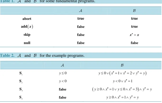
Four fundamental programs are abort, add x

( )

, skip and null for which the corresponding formulae are given in Table 1. From this table we see that:

( )

≤ ≤ ≤

abort add x skip null

when x is non-empty, then all three refinements are strict refinements. Note that abort and add x

( )

have the same behaviour but different termination conditions, while add x

( )

and skip have the same termination conditions but different behaviour. (When x is empty add

( )

is equivalent to skip and the formula

′′ ≠

x x is equivalent to true.)

Examples

Some example programs to illustrate the formulae:

{

} (

)

1= y>0 ; x: 1= x: 2=

S 

{

}

2= y≥0 ; x: 1=

S

3 = y≥ → =0 x: 1 y≤ → =0 x: 3

S if  fi

[

]

4 = y≥0 ; x: 1=

S

Here, S₂ is both more defined (terminating on more initial states) and more deterministic than S₁, and so

2

S is a refinement of S₁. A refinement of a program can define any behaviour for initial states on which the original program aborts, so S₃ is also a refinement of S₁. Finally, S₄ is more deterministic than S₃ in that it restricts the set of possible final states (for initial states with y<0 the set of final states is empty).

These facts are reflected in the formulae in Table 2.

Clearly, 

( )

S2 ⇒

( )

S1 and 

( )

S2 ⇒

( )

S1 which shows that S1≤S2. Also 

( )

S3 ⇒

( )

S1 and

( )

S3 ⇒

( )

S1

  which shows that S₁≤S₃. However, it is not the case that S₂ ≤S₃ since when y=0 in- itially, S₂ must assign x the value 1, while S₃ can non-deterministically choose to assign x the value 1 or 3. Conversely, S₃ is not refined by S₂ because S₃ is defined on initial states for which S₂ is not de-fined: namely, those initial states in which y<0.

Finally, S₄ is a (strict) refinement of all the other programs, and none of the other programs is a refinement of S₄ because S₄ is null on initial states with y<0.

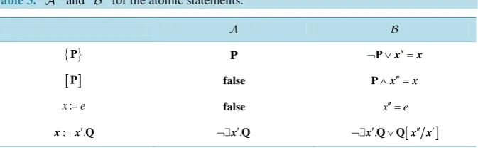
[image:5.595.127.472.503.721.2]

Given that  and  capture the semantics of a program, it should be possible to compute the formulae for a compound statement from the formulae for the components. For the primitive statements in the first level of WSL, the formulae are given in Table 3.

Table 1.  and  for some fundamental programs.

 

abort true true

( )

add x false true

skip false x′′ =x

null false false

Table 2.  and  for the example programs.

 

1

S y≤0 y≤ ∨0 (x′′= ∨1 x′′= ∨2 y′′=y)

2

S y<0 y< ∨0 x′′=1

3

S false (y≥ ∧0 x′′= ∨ ≤ ∧1 y 0 x′′= ∧3) y′′=y

4

[image:5.595.127.469.504.721.2]

(6)

[image:6.595.132.469.91.195.2]

Table 3.  and  for the atomic statements.

 

{ }P P ¬ ∨P x′′=x

[ ]

P false P∧x′′=x

:

x=e false x′′ =e

:= ′.Q

x x ¬∃x′.Q ¬∃x′.Q∨Q

[

x x′′ ′

]

4. Computing



and



for Compound Statements

Given the two formulae 

( )

S and 

( )

S , which are in effect, the weakest preconditions on S for two particular postconditions, we can determine the weakest precondition for any given postcondition. This means that we can compute  and  for any compound statement, given the corresponding formulae for the compo- nent statements.

For nondeterministic choice:

(

)

(

)

(

)

(

)

(

)

(

)

( )

1 2 1 2

1 2

WP ,

WP , WP ,

⇔ ¬

⇔ ¬ ∧

⇔ ¬ ∨ ¬

⇔ ∨

S S S S true

S true S true S true S true

S S

 



 

and similarly:

(

S1S2

)

⇔

( )

S1 ∨

( )

S2

  

For deterministic choice:

(

)

(

)

(

)

(

)

(

)

(

)

(

)

(

)

( )

(

)

(

( )

)

1 2 1 2 1 2 1 2

WP , WP ,

⇔ ¬ ⇒ ∧ ¬ ⇒

⇔ ∧ ¬ ∨ ¬ ∧ ¬

⇔ ∧ ∨ ¬ ∧

if B then S else S fi

B S true B S true

B S B S



 

and similarly:

(

)

( )

(

1 1

)

(

2

( )

2

)

⇔ ∧ ∨ ¬ ∧

if B then S else S fi

B S B S



 

For sequential composition:

(

)

(

)

( )

(

)

( )

(

( )

( )[

]

)

(

)

( )

(

( )

( )[

]

)

1 2 1 2

1 2

1 1 1 2

; WP , WP ,

WP , . . . . ⇔ ¬ ⇔ ¬ ¬ ′′ ′′ ′′ ⇔ ¬ ¬∃ ∨ ¬ ∧ ∀ ⇒ ¬ ′′ ′′ ′′ ⇔ ∃ ∧ ∨ ∃ ∧

S S S S true

S S

S S S S



   

x x x x

In other words, for S S₁; ₂ to abort on an initial state, S₁ must not be null and either S₁ aborts or S₁ terminates in a state in which S₂ aborts.

To compute 

(

S S₁; ₂

)

we need to compute WP

(

S₁, WP

(

S₂,x≠x′′

)

, but this contains a postcondition which includes variables in x′′ . We can solve this problem by computing the formula

(

)

(

1 2

)

WP S , WP S ,x≠x′ and then renaming x′ to x′′ in the result. Note that the postcondition

(

2

)

(7)

561

(

)

(

)

[

]

( )[

]

(

)

[

]

( )

(

( )

( )[

][

]

)

(

)

[

]

( )

(

( )

(

( )

( )[

][

]

)

[

]

( )

(

( )

(

( )[

]

( )[

]

)

1 2 1 2

1 2

1 1 1 2

; WP , WP ,

WP ,

. .

′ ′′ ′

⇔ ¬ ≠

′ ′′ ′′ ′

⇔ ¬ ¬

′′ ′′ ′ ′′ ′′ ′′ ′

⇔ ¬ ¬∃ ∨ ¬ ∧ ∀ ⇒ ¬

′′ ′′ ′ ′′ ′′ ′′ ′

⇔ ∃ ∧ ∨ ∃ ∧

′′ ′ ′ ′′ ′

⇔ ∃ ∧ ∨ ∃ ∧

S S S S

S S

S S S S



   

x x x x

x x x x

x x x x x x x x

x x x x x x

In other words, for x′′ to be a possible final state for S S₁; ₂ on initial state x, either S₁ aborts or there exists some intermediate state x′ which is a possible final state for S₁ and for which S₂ gives x′′ as a possible final state when started in this initial state.

Recursion

(

µXx.S

)

y is defined in terms of the set of all finite truncations. Define:

(

)

0

( )

DF

. ; ;

X

µ yxS = abort add x remove y

(

)

1

(

)

DF

. n . n forall

X X X n

µ + = _ µ _ <ω

 

S S S

x x

y y

Then for any postcondition R:

(

)

(

)

DF

(

)

WP . , . n,

n

X X

ω

µ µ

<

=

∨

S R S R

x x

y y

So:

(

)

(

.

)

(

.

)

n

)

and

(

.

)

(

.

)

n

)

n n

X X X X

ω ω

µ µ µ µ

< <

≡

∧

≡

∧

S S S S

 x  x  x  x

y y y y

5. Temporal Logic

Temporal logic [3] is a class of logical theories for reasoning about propositions qualified in terms of time and can therefore be used to reason about finite and infinite sequences of states. These sequences can define an operational semantics for programs which maps each initial state to the set of possible histories: where a history is a possible sequence of states in the execution of a program. Since a formula can describe an infinite sequence of states: and therefore a non-terminating program, there would appear to be no need for the special state ⊥ to indicate non-termination, and therefore it would appear possible to represent the operational semantics of a program using a single formula in temporal logic.

This turns out not to be the case: a single formula is not sufficient, but two formulae (the temporal equivalent of the abort and behaviour predicates defined here) are sufficient. Lack of space precludes a full discussion of these questions in this paper.

References

[1] Ward, M. (2004) Pigs from Sausages? Reengineering from Assembler to C via Fermat Transformations. Science of Computer Programming, Special Issue on Program Transformation, 52, 213-255.

http://www.gkc.org.uk/martin/papers/migration-t.pdf

[2] Dijkstra, E.W. (1976) A Discipline of Programming. Prentice-Hall, Englewood Cliﬀs.