A Comparative Algorithmic Approach to Predict Probability of Fault in a Module by Indirect Coupling

(1)

A Comparative Algorithmic Approach to Predict

Probability of Fault in a Module by Indirect Coupling

Kireet Joshi

M.Tech Scholar, Computer Science & Engineering

B.T.K.I.T, Dwarahat

Ramesh Chandra Belwal

Asst. Professor, Deptt. Of Computer Science & Engineering

B.T.K.I.T, Dwarahat

Shailendra Mishra,

PhD. Prof. & H.O.D, Computer Science &

Engineering B.T.K.I.T, Dwarahat

ABSTRACT

Any defect in the software module or a project can hamper the quality of software projects that leads to failure of the projects, so prediction of defects is a very important task in the development of software development life cycle (SDLC).In this research paper an algorithmic approach is proposed that will compare the probability of defects due to indirect coupling in the software modules with respect to direct coupled modules. Since the indirect coupling in the software modules can be find out by taking the transitive closure between different modules, but predicting the probability of defects in the software modules via direct coupling is always been a tough task for the programmers, as there may be various hidden dependencies which cannot be exactly detected by direct coupling between software modules. So this paper provides an extension of the previous work done on direct coupled modules, for finding increased probability of defects or faults between dependent modules by indirect coupling approach.

Keywords

Defect Prediction using Indirect Coupling, Fault detection, Coupling, Fault Localization, Software Quality, Defects

1. INTRODUCTION

Reducing high Dependency in the software modules has always been a challenging task for the programmers in order to make an efficient and reliable system that is completely free from defects. In software engineering, coupling or dependency means how each module or a program fragment is related with each other. The type of coupling which have been in little attention is indirect coupling [8][9],which is coupling between software modules that are indirectly related. Efforts are made to create a model that serve low coupling and high cohesion and is reusable.One can’t have modules in the system that is completely independent of each other. They must interact with each other so that the exchange of information between them is maintained. Various past researches have been done that focuses on direct coupling which is a form of coupling that exists between modules that are directly related to each other. Excessive coupling[11][12] between software modules deteriorates the important property of object oriented design i.e. reusability, and there is increased chance that it will also cause the modularity of the software to hamper. To improve modularity and other properties of object oriented system one must have the effect of coupling as low as possible so as to obtain lesser number of defects. Coders and testers always make an effort to improve the

zero or minimum defects. There may be some modules or components that produce high risk in the software project and should be detected as early as possible so that software’s quality should be enhanced before it is delivered to the customer’s site. Defects in the software or module always results in cost in terms of quality and time. Also it should be kept in mind that it is not practically possible to eliminate each and every defect in the software module or in project but the intensity and the magnitude of the defects can be minimised before it is delivered or made operational[1].

2. DEFECT PREDICTION

Software Defect is any flaw in the software development life cycle that would produce unexpected results as compared to the actual results and would cause that software or the project to fail to meet the desired requirements in software development process. A defect generally represents unwanted results in the software that hampers software quality. There exists network metrics on code entity dependency graphs [5] that can be used to build some defect prediction models. Afterwards the set of network metrics were extended [6] by extending code dependency graph adding contribution dependency edges.

As defect prediction is a relatively a new area of research. Almost in every software engineering projects, knowledge discovery is applied by the testing team by gaining the information about the data which is collected, and defect detection process is applied by concentrating more on the affected modules that are fault prone and analysis is done so that in near future the probability of defects in similar modules or projects can be minimised. With the importance of enforcing the highest levels of quality in software models, it has become an important task for the development team to improve defect prediction techniques so that greater number of defects can be minimised in little span of time with improved efficiency and reliability before the software is delivered to the customers site.

When the software faults are analyzed by the project team in some modules then some efficient fault localization[7] algorithms should be applied so that cost and time factors should be reduced [2].To enhance software’s quality, the project team have to emphasize more on how maximum number of defects can be removed in less amount of time without introducing some new bugs or defects in the system.

3. RELATED WORK

(2)

longer the two modules are connected to each other the more hidden dependence. Indirect coupling can also be analyzed and detected by the transitive closure of the modules, but there may be some circumstances that instead of transitive closure the indirect coupling may still exist and leads

hidden modules undetected in software engineering process[3].

The existing algorithm calculates the Defect Propagation factor [13] to find the probability of the dependent modules to be fault prone by direct coupling. Indirect approach gives an increased probability of defect detection in the program or software module [4].

4. PROPOSED APPROACH

Some abbreviations that are used throughout in the paper for calculations:

Calculate the indirect coupled defect propagation factor (IDFxz) =

𝒄𝒐𝒎𝒎𝒐𝒏 𝒅𝒆𝒇𝒆𝒄𝒕 𝒑𝒓𝒐𝒅𝒖𝒄𝒊𝒏𝒈 𝒗𝒂𝒓𝒊𝒂𝒃𝒍𝒆𝒔 𝒃𝒆𝒕𝒘𝒆𝒆𝒏 𝒊𝒏𝒅𝒊𝒓𝒆𝒄𝒕𝒍𝒚 𝒍𝒊𝒏𝒌𝒆𝒅 𝒅𝒆𝒑𝒆𝒏𝒅𝒆𝒏𝒕 𝒎𝒐𝒅𝒖𝒍𝒆𝒔

𝒄𝒐𝒎𝒎𝒐𝒏 𝒗𝒂𝒓𝒂𝒊𝒃𝒍𝒆𝒔 𝒃𝒆𝒕𝒘𝒆𝒆𝒏 𝒊𝒏𝒅𝒊𝒓𝒆𝒄𝒕 𝒍𝒊𝒏𝒌𝒆𝒅 𝒅𝒆𝒑𝒆𝒏𝒅𝒆𝒏𝒕 𝒎𝒐𝒅𝒖𝒍𝒆𝒔

And Percentage Defect propagation factor [13] DFxz is given by

𝒅𝒆𝒇𝒆𝒄𝒕 𝒑𝒓𝒐𝒅𝒖𝒄𝒊𝒏𝒈 𝒗𝒂𝒓𝒊𝒂𝒃𝒍𝒆𝒔 𝒑𝒂𝒓𝒕𝒊𝒄𝒊𝒑𝒂𝒕𝒊𝒏𝒈 𝒃𝒆𝒕𝒘𝒆𝒆𝒏 𝒅𝒆𝒑𝒆𝒏𝒅𝒆𝒏𝒕 𝒎𝒐𝒅𝒖𝒍𝒆𝒔 𝒄𝒐𝒎𝒎𝒐𝒏 𝒗𝒂𝒓𝒊𝒂𝒃𝒍𝒆𝒔 𝒃𝒆𝒕𝒘𝒆𝒆𝒏 𝒅𝒆𝒑𝒆𝒏𝒅𝒆𝒏𝒕 𝒎𝒐𝒅𝒖𝒍𝒆𝒔

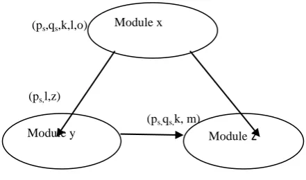
(ps,qs,k,l,o)

(ps,l,z)

[image:2.595.56.277.359.489.2]

(ps,qs,k, m)

Fig 1: Direct and Indirect Coupled Modules

Suppose from the above figure, there is a set of interlinked modules such that one of the modules is interdependent on another. Let CDxy consists of common variables between modules x and y.CDxz consist of common variables between modules x and z.CDyz consist of common variables between modules y and z.Let DVxy be the set of defect producing variables participating between dependent modules(x and y).DVyz be the set of defect producing variables participating between dependent modules (y and z). The intent is to find the probability of the module to be fault prone with indirect coupling.

If the Indirect coupled Defect Propagation Factor IDFxz, exceeds the Defect Propagation Factor DFxz, then it can be said that the module having high Indirect coupled Defect Propagation Factor with respect to Defect Propagation Factor is statistically more fault prone, and the dependency (interdependency) is higher or more hidden dependence is there. So it will help the testing team to focus more on that defected module for further debugging and their efficiency increases.

4.1. Proposed Algorithm

Input –

All variables in each module.

All defect producing variables propagating in dependent modules.

Output: Set of more fault prone indirectly linked dependent module as compared to directly coupled modules.

Method:

For each module Mx, get the set of dependent modules // where x=1 to n

For each module My, Where y=1 to n

/* This for loop constitutes set of variables present in module and compares them with the variables present in dependent set of modules */

{

For each directly dependent module Mz // where z=1 to n and x≠z

{

Find CDxz, where CDxz is the set of common variables between the dependent modules.

/* CDxz [13] is calculated by taking the intersection of the variables from the dependent set of modules */

} }

For each module Mx // where x=1 to n {

/* This for loop accounts for set of variables along with the variables that are responsible in producing defects and compares them with the variables present in dependent set of modules */

For every dependent module Mz //where z≠x

{

Find DVxz, where DVxz is the set of defect producing variables participating in the directly linked dependent modules and are responsible for producing defects.

/* DVxz is calculated by taking the intersection of the variables that are participating in the dependent modules and are responsible for producing defects */

Calculate percentage Defect propagation factor [13] (DFxz) of directly linked dependent modules =

𝒅𝒆𝒇𝒆𝒄𝒕 𝒑𝒓𝒐𝒅𝒖𝒄𝒊𝒏𝒈 𝒗𝒂𝒓𝒊𝒂𝒃𝒍𝒆𝒔 𝒑𝒂𝒓𝒕𝒊𝒄𝒊𝒑𝒂𝒕𝒊𝒏𝒈 𝒃𝒆𝒕𝒘𝒆𝒆𝒏 𝒅𝒆𝒑𝒆𝒏𝒅𝒆𝒏𝒕 𝒎𝒐𝒅𝒖𝒍𝒆𝒔 𝒄𝒐𝒎𝒎𝒐𝒏 𝒗𝒂𝒓𝒊𝒂𝒃𝒍𝒆𝒔 𝒃𝒆𝒕𝒘𝒆𝒆𝒏 𝒅𝒆𝒑𝒆𝒏𝒅𝒆𝒏𝒕 𝒎𝒐𝒅𝒖𝒍𝒆𝒔

} }

For each module Mx // where i=x 1 to n {

For every dependent module My // where y=1 to n x≠y {

Module x

(3)

For every indirectly linked module Mz which is coupled directly with every dependent module My// where z=1 to n and z≠y

{

Find the indirect coupled defect propagation factor ( IDFxz)=

If (IDFxz) >= (DFxz)

/*Where (DFxz) is calculated above as

𝒅𝒆𝒇𝒆𝒄𝒕 𝒑𝒓𝒐𝒅𝒖𝒄𝒊𝒏𝒈 𝒗𝒂𝒓𝒊𝒂𝒃𝒍𝒆𝒔 𝒑𝒂𝒓𝒕𝒊𝒄𝒊𝒑𝒂𝒕𝒊𝒏𝒈 𝒃𝒆𝒕𝒘𝒆𝒆𝒏 𝒅𝒆𝒑𝒆𝒏𝒅𝒆𝒏𝒕 𝒎𝒐𝒅𝒖𝒍𝒆𝒔

𝒄𝒐𝒎𝒎𝒐𝒏 𝒗𝒂𝒓𝒊𝒂𝒃𝒍𝒆𝒔 𝒃𝒆𝒕𝒘𝒆𝒆𝒏 𝒅𝒆𝒑𝒆𝒏𝒅𝒆𝒏𝒕 𝒎𝒐𝒅𝒖𝒍𝒆𝒔

Then, there is probability that indirectly linked dependent module is more fault prone as compared to directly linked coupled module and there may be some hidden dependencies between the modules.

Else

Probability of hidden dependencies is low between the coupled modules

} } }

From the proposed algorithm if the Indirect coupled defect propagation factor is greater than the Defect Propagation Factor [13] (directly coupled) then the probability of the module to be fault prone increases and there are some hidden dependencies and testing team have to focus more on checking that particular fault prone modules, so that the defect should not propagate in the whole system.

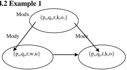
4.2 Example 1

Modx

Mody Modz

.

Some abbreviations that are use in the paper for calculating tasks:

Defect Propagation factor (DF) [13] between the set of dependent modules =

𝒅𝒆𝒇𝒆𝒄𝒕 𝒑𝒓𝒐𝒅𝒖𝒄𝒊𝒏𝒈 𝒗𝒂𝒓𝒊𝒂𝒃𝒍𝒆𝒔 𝒑𝒂𝒓𝒕𝒊𝒄𝒊𝒑𝒂𝒕𝒊𝒏𝒈 𝒃𝒆𝒕𝒘𝒆𝒆𝒏 𝒅𝒆𝒑𝒆𝒏𝒅𝒆𝒏𝒕 𝒎𝒐𝒅𝒖𝒍𝒆𝒔

𝒄𝒐𝒎𝒎𝒐𝒏 𝒗𝒂𝒓𝒊𝒂𝒃𝒍𝒆𝒔 𝒃𝒆𝒕𝒘𝒆𝒆𝒏 𝒅𝒆𝒑𝒆𝒏𝒅𝒆𝒏𝒕 𝒎𝒐𝒅𝒖𝒍𝒆𝒔

Indirect coupled Defect Propagation Factor (IDF) between the modules =

For example, consider three modules as per the given figure and try to find out the probability of fault prone module.

Let x={ps,qs,r,k,o,}and y= { ps,qs,r,w,u }are set of variables

in Module x and Module y // where ps,qs are the variables

producing defects.

CDxy= { ps,qs,r } are set of common variables between the

dependent set of modules x and y [13].

DVxy= { ps,qs },where DVxy is the set of defect producing

variables participating in the dependent modules.

Defect propagation factor (DFxy) =2/3 or 66.66 %( or in other words it can be said that if module x is producing defect than statistically it could be said that there is approximate 66.66% probability, module y would also produce defect).

Let y={ ps,qs,r,w,u } z={ps,qs,t,k,o}be the set of variables in

modules y and z.

CDyz= { ps,qs } be the set of common variables between the

dependent set of modules y and z.

DVyz= { ps,qs} is the set of defect producing variables

participating in the dependent modules.

Defect propagation factor (DFyz) =2/2 or 100%( or in other words it can be said that if module y is producing defect than statistically there is approximate 100% probability, module z would also produce defect).

Let x={ ps,qs,r,k,o,} z={ ps,qs,t,k,o}are set of variables in

modules x and z.

CDxz= { ps,qs,k,o } be the set of common variables between

the dependent set of modules x and z.

DVxz={ ps,qs } is the set of defect producing variables

Defect propagation factor (DFxz) =2/4 or 50%(or in other words it can be said that if module x is producing defect than statistically there is approximate 50% probability , module z would also produce defect).

Now, the Indirect Coupled Defect Propagation Factor between modules x and z is calculated by taking the ratio of common defect producing variables participating in all modules to the common variables between the indirectly linked set, i.e.(IDFxz)=2/2 or 100%,it means statistically the probability that module z is fault prone is high when indirect coupling is considered as compared to defect propagation factor (direct) DFxz=50%.

4.2. Example 2

Modx

[image:3.595.57.268.440.556.2]

Modz Mody

For example, consider three modules as per the given figure and try to find out the probability of fault prone module. {ps,qs,r,k,o,}

{ps,qs,r,w,u} {ps,qs,t,k,o}

{ms,ns,ps,v,l}

(4)

Let x={ ms,ns,ps,v,l }and y={ ms,ns,v }are set of variables in

Module x and Module y // where ms,ns,ps are the variables

producing defects.

CDxy= { ms,ns,v }are set of common variables between the

dependent set of modules x and y.

DVxy= { ms,ns },where DVxy is the set of defect producing

Defect propagation factor (DFxy) =2/3 or 66.66 %(or in other words ,it can be said that if module x is producing defect than statistically it could be said that there is approximate 66.66% probability , module y would also produce defect).

Let y={ ms,ns,v } z={ ms,ns,ps,w,u,v }be the set of variables

in modules y and z.

CDyz= { ms,ns,v } be the set of common variables between

the dependent set of modules y and z.

DVyz= {ms,ns} is the set of defect producing variables

Defect propagation factor (DFyz) =2/3 or 66.66 %( or in other words, it can be said that if module y is producing defect than statistically there is approximate 66.66% probability, module z would also produce defect).

Let x={ ms,ns,ps,v,l } z={ ms,ns,ps,w,u,v }are set of variables

in modules x and z.

CDxz= { ms,ns,ps,v } be the set of common variables between

DVxz={ ms,ns,ps } is the set of defect producing variables

Defect propagation factor (DFxz) =3/4 or 75 %(or in other words it can be said that if module x is producing defect than statistically there is approximate 75% probability , module z would also produce defect ) .

Now,the Indirect Coupled Defect Propagation Factor between modules x and z is calculated by taking the ratio of common defect producing variables participating in all modules to the common variables between the indirectly linked set, i.e. (IDFxz) =2/3 or 66.66%, it means statistically the probability that module z is more fault prone as compared to defect propagation factor DFxz=75% (direct) is less and there may not be any hidden dependencies in the module.

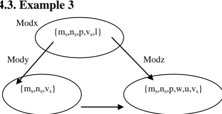
4.3. Example 3

Modx

Mody Modz

For example, consider three modules as per the given figure and try to find out the probability of fault prone module. Let x={ ms,ns,p,vs,l }and y={ ms,ns,vs }are set of variables in

Module x and Module y // where ms,ns,vs are the variables

producing defects.

CDxy= { ms,ns,vs }are set of common variables between the

dependent set of modules x and y.

DVxy= { ms,ns,vs },where DVxy is the set of defect producing

Defect propagation factor (DFxy) =3/3 or 100%(or in other words, it can be said that if module x is producing defect than statistically it could be said that there is approximate 100% probability , module y would also produce defect).

Let y={ ms,ns,vs } and z={ ms,ns,p,w,u,vs } be the set of

variables modules y and z.

CDyz= { ms,ns,vs } be the set of common variables between

the dependent set of modules y and z.

DVyz= { ms,ns,vs } is the set of defect producing variables

Defect propagation factor (DFyz) =3/3 or 100 %( or in other words, it can be said that if module y is producing defect than statistically there is approximate 100% probability, module z would also produce defect).

Let x={ ms,ns,p,vs,l } z={ ms,ns,p,w,u,vs }are set of variables

in modules x and z.

CDxz= { ms,ns,p,vs } be the set of common variables between

DVxz={ ms,ns,vs } is the set of defect producing variables

participating in the dependent modules. Defect propagation factor (DFxz) =3/4 or 75%(or in other words, it can be said that if module x is producing defect than statistically there is approximate 75% probability , module z would also produce defect ) Now, the Indirect Coupled Defect Propagation Factor between modules x and z is calculated by taking the ratio of common defect producing variables participating in all modules to the common variables between the indirectly linked set,i.e.(IDFxz)=3/3 or 100%,it means statistically the probability that module z is highly fault prone as compared to defect propagation factor DFxz=75% (direct) increases and there may be hidden dependencies in the module.

[image:4.595.56.276.556.669.2]

5. RESULTS & COMPARISION

Table 1: Results of Proposed approach showing relation between of the probability fault prone modules and

dependencies

Dependent modules

Defect Propagat

ion Factor(

%)

Indirect Coupled Defect Propogatio

n Factor(%)

Probability of Indirectly

coupled modules to

be fault prone

Possibilit y of Hidden depende ncies

(x,y) 66.66 - - -

(x,z) 50 100 high high

(y,z) 100 - - -

{ms,ns,p,vs,l}

(5)

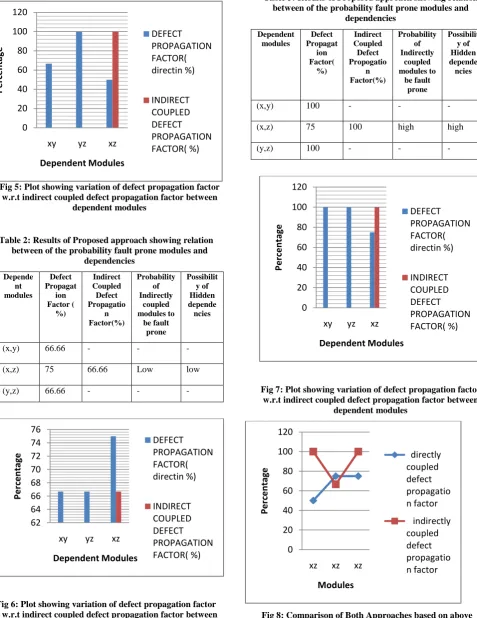
Fig 5: Plot showing variation of defect propagation factor w.r.t indirect coupled defect propagation factor between

[image:5.595.37.282.77.259.2]

dependent modules

dependencies

Depende nt modules

ion Factor (

%)

Indirect Coupled Defect Propagatio

n Factor(%)

(x,y) 66.66 - - -

(x,z) 75 66.66 Low low

(y,z) 66.66 - - -

dependencies

Dependent modules

ion Factor(

%)

Indirect Coupled Defect Propogatio

n Factor(%)

(x,y) 100 - - -

(x,z) 75 100 high high

[image:5.595.57.535.80.699.2]

(y,z) 100 - - -

Fig 8: Comparison of Both Approaches based on above examples in Predicting higher probability of a module to

be fault prone and hidden dependencies between them

62 64 66 68 70 72 74 76

xy yz xz

Per

ce

n

tage

Dependent Modules

DEFECT PROPAGATION FACTOR( directin %)

INDIRECT COUPLED DEFECT PROPAGATION FACTOR( %)

0 20 40 60 80 100 120

xy yz xz

Per

ce

n

tage

INDIRECT COUPLED DEFECT PROPAGATION FACTOR( %)

0 20 40 60 80 100 120

xz xz xz

P

er

ce

n

tag

e

Modules

directly coupled defect propagatio n factor

indirectly coupled defect propagatio n factor 0

20 40 60 80 100 120

xy yz xz

Per

ce

n

tage

[image:5.595.306.543.90.440.2] [image:5.595.51.278.347.664.2]

(6)

From the above results it may be concluded that the testing team will now focus more on module k as there may be some hidden dependencies that may not be detected by considering only the directly coupled modes, and this will give an idea to the testing team members to focus more on the defects that are caused by indirectly coupled modules. Greater the Indirect coupled defect propagation factor than defect propagation factor [13] (direct), there will be an increased probability of the module to be fault prone. And as a result more defects can be located. For any module the coupling whether it is direct or indirect it should be as minimum as possible for a system to be free from any kind of defects. If the indirect coupled propagation factor is more it means there are some hidden dependencies between the modules which may not be detected by taking direct coupled modules alone.

6

.

CONCLUSION

The paper focuses the application knowledge discovery in predicting the probability of fault prone module in indirectly linked software modules. The proposed paper demonstrates an algorithmic approach for indirectly coupled interlinked software modules in comparison to directly coupled modules so that there will be higher chances for the testing team to detect the fault prone module as more effort is required in detecting defects in indirectly coupled modules. This will give an ease to the project team members to efficiently analyze the higher probability modules for defects and to make more reliable and cost efficient models for software industry in less time.

7. REFERENCES

[1] Tan, Xi Sch. of Comput. Sci., Fudan Univ., Shanghai, China Peng, Xin, Pan, Sen, Zhao, Wenyon,” Assessing Software Quality by Program Clustering and Defect Prediction”, Reverse Engineering (WCRE), 2011 18th Working Conference,pp. 244 – 248, Oct. 2011,ISSN : 1095-1350.

[2] Gonzalez-Sanchez, Alberto Software Technol. Dept., Delft Univ.of Technol.,Delft,Netherlands Abreu, Rui, Gross, Hans-Gerhard, Van Gemund, Arjan J C,” Prioritizing tests for fault localization through ambiguity group reduction”, Automated Software Engineering (ASE), 2011 26th IEEE/ACM International Conference, pp. 83 – 92,6-10 Nov. 2011, ISSN : 1938-4300. [3] Vinay Singh and Vandana Bhattacherjee,” Detection of

Indirect Coupling Using Chaining Method and Its Impact on Software Quality”, International Journal of Research and Reviews in Information Sciences (IJRRVol. 1, No. 4, December 2011, ISSN: 2046-6439.

[4] Jalbert, Kevin Software Quality Res. Group, Univ. of Ontario Inst. of Technol., Oshawa, ON, Canada

Bradbury, Jeremy S.,” Using clone detection to identify bugs in concurrent software”, Software Maintenance (ICSM), 2010 IEEE International Conference,pp. 1 – 5, 12-18 Sept. 2010, ISSN : 1063-6773.

[5] T. Zimmermann and N. Nagappan, “Predicting defects using network analysis on dependency graphs,” in Proceedings of the 30th international conference on Software engineering, ser. ICSE ’08. ACM, 2008, pp.531–540.

[6] C. Bird, N. Nagappan, H. Gall, B. Murphy, and P. Devanbu, “Puttingit all together: Using socio-technical networks to predict failures,” in Proceedings of the 2009 20th International Symposium on Software Reliability Engineering, ser. ISSRE ’09. IEEE Computer Society, 2009,pp. 109–119.

[7] Liu Yanbin Ordnance Eng. Coll., Shijiazhuang, China,Zhu Xiaodong,Sun Zhiming,Wang Yigang,Ye Fei,” Dual-Slices Algorithm for Software Fault Localization”, Computational Intelligence and Software Engineering, 2009. CiSE 2009. International Conference, pp. 1 – 4, 11-13 Dec. 2009, Print ISBN: 978-1-4244-4507-3.

[8] Yang H. and Tempero E., 2007, Indirect Coupling as a Criteria for Modularity. In Proceedings of the First International Workshop on Assessment of Contemporary Modularization Techniques (ACoM '07). IEEE ComputerSociety, Washington, DC, USA, 10-11. [9] Yang H. and Tempero E., 2007, Measuring the Strength

of Indirect Coupling, In Proceedings of the 2007 Australian Software Engineering Conference (ASWEC '07). IEEE Computer Society, Washington, DC, USA, 319-328.

[10] N. DiGiuseppe and J. Jones. On the inﬂuence of multiple faults on coverage-based fault localization. In Proceedings of the 9th ACM/IEEE International Symposium on Software Testing and Analysis, ISSTA ’11, page To Appear, New York, NY, USA, 2011. ACM.

[11] Briand,L.C., Daly,J.W., & Wust,J.K.,”A Unified framework for coupling measurement in object oriented system”. IEEE Transact Software Engineering, (25(1): pp. 91-121, January/February 1999.

[12] Yourdon. & Constantine, L.L,” Structured Design: Fundamental of a discipline of computer program and system design prentice hall”, 1979.