Energy Efficient Hierarchical Routing Protocol (EEHRP)
for Wireless Sensor Network
Rajendra S. Bisht
Assistant Professor Graphic Era Hill University Bhimtal, Uttarakhand, India
Manoj Chandra Lohani,
Ph.D Associate Professor Graphic Era Hill University Bhimtal, Uttarakhand, IndiaSandeep K. Budhani
Assistant Professor Graphic Era Hill University Bhimtal, Uttarakhand, India
ABSTRACT
Wireless sensor network consisting of various tiny wireless sensor nodes that are equipped with transmission devices that require some amount of energy to transmit the data to other node(s). Most often the battery of sensor nodes cannot be charged or changed during transmission. To preserve the longetivity of the network it is very challenging task to build a sensor node that require very little amount of energy for data transmission. Lifetime of wireless sensor network is directly proportional to the energy source of wireless sensor node. It is proved that 70% of energy consumption is caused during data transmission process [1]. In order to maximize the network lifetime we need to optimize data transmission process. An energy efficient routing algorithm may result in better network lifetime. This is the reason why routing techniques in wireless sensor network focus mainly on the accomplishment of power conservation. Most of the recent researches have shown various algorithms mainly designed to minimize energy consumption in sensor networks. Each routing mechanism has its advantages and disadvantages over energy efficiency. There is no single, best routing protocol that is suitable for all applications. Routing mechanism might differ depending on the application, network architecture and topologies. Routing algorithms/techniques have been classified in a number of ways by various researchers. There is no general classification is available till today. Some researchers [2, 3, 4, and 5] have classified routing algorithms into three broad categories Data-centric Routing Protocols, Hierarchical Routing Protocols and Location-based Routing Protocols. In this Paper an energy efficient hierarchical routing algorithm is being proposed. Using simulation a basic idea is also given in this paper that shows how hierarchical routing mechanism is better than non hierarchical mechanism.
Keywords
Base station (sink), Clustering, Energy efficiency, Routing Protocols, CH (Cluster Head), Wireless Sensor Network
1.
INTRODUCTION
A Wireless Sensor Network (WSN) is a collection of various tiny nodes (called sensors) densely deployed in a small or large geographical area. WSNs are used in various applications such as civil, army, security to monitor physical or environmental conditions. Sensor nodes in WSN also can be considered as a collection of low-cost, low-power, and multifunctional wireless sensor nodes. A sensor node is capable of sensing temperature, air pressure, atmosphere, sound etc. In a WSN a collection of wireless sensor nodes are responsible for gathering data from environment. Gathered data is then sent to the base station for data processing to conclude some information. The process of sending data from all sensor nodes to base station will result in energy wastage due to redundant data transmission. For a large geographical area it may not be possible to transmit data
directly to base station. To overcome these issues we adopt some data gathering and data aggregation mechanism to routing algorithms.
2.
WORKING OF PROPOSED
ALGORITHM
In this Paper an algorithm “EEHRP- ENERGY EFFICIENT HIERARCHICAL ROUTING PROTOCOL” is proposed that is much energy efficient. This algorithm is based on hierarchical routing technique that involves clustering of sensor nodes. Clustering in WSNs is grouping of sensor nodes in large scale sensor network. At very first stage of algorithm all sensor nodes form clusters within WSN. In next stage Cluster Head selection took place in each cluster. These cluster heads are responsible for gathering data from sensor nodes within their cluster. Cluster head from each cluster aggregate gathered data and send it to another cluster head or to the Base station (sink) depending on the distance between them (lower distance is considered) . As compare to the technique in which each sensor node was responsible for sending data directly to the base station, this technique saves much more energy. After the completion of a particular round Cluster head selection algorithm rotates the cluster head by estimating the residual energy in each sensor node within a cluster. The distance between communicating nodes is also considered. According to system energy model in figure 1 energy required to transmit data is different according to the distance between communicating nodes. This rotation of cluster head uniforms the energy consumption of sensor nodes.
3.
SYSTEM ENERGY MODEL OF A
SENSOR NODE
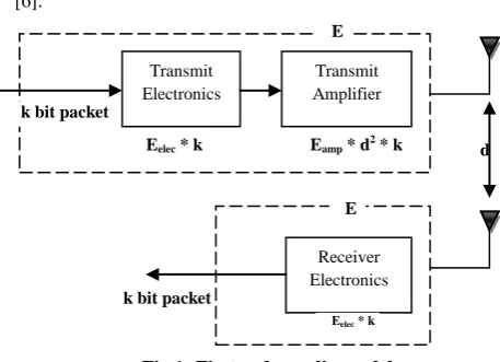
[image:1.595.303.532.582.747.2]Having an understanding that the wireless communication component of a sensor node is responsible for the energy draining activities, we use the radio model shown in Figure 1 [6].
Fig 1: First order radio model
d
k bit packet
Transmit Electronics Transmit Amplifier Receiver Electronics
k bit packet
Eamp * d2 * k
Eelec * k
Eelec * k
13 The first order radio model offers an evaluation of energy
consumed when transmission or reception is made by a sensor node at each cycle. The radio has a power control to expend minimum energy required to reach the intended recipients. Mathematically, when a k-bit message is transmitted through a distance, d, required energy can be expressed as stated in the equation:
Energy required to transmit Data ETx = Eelec * k + Eamp * d
2
* k (1) Energy consumed at the reception
ERx =Eelec * k (2)
Where
Eelec - Cost of circuit energy when transmitting or receiving one
bit of data
Eamp - Amplification factor
k - a number of transmitted data bits D - distance between sender and receiver
4.
ENERGY EFFICIENT
HIERARCHICAL ROUTING
PROTOCOL (EEHRP)-THE
PROPOSED ROUTING PROTOCOL
ALGORITHM
The algorithm consists of five main Steps
1. Formation of M Clusters (where M is integer). Repeat Step 2,3, 4 for ‘R’ Rounds (where R is an integer). 2. Cluster Head Selection for each cluster( see below for
detail working)
3. Data Aggregation phase–In this phase Cluster head collects the data from Wireless sensor nodes or from other Cluster Head.
4. Data transmission phase- In this phase Cluster Head transfers all data to Base Station.
5.
CLUSTER HEAD SELECTION
ALGORITHM
A. Einitial(n) i.e initial energy is measured
B. d(n) is measured i.e. min( distance from each node to the base station , distance to the corresponding higher level cluster head )
C. (Eamp*k*d 2
) is the energy required by each node for transmission.
D. The maximum energy after the subsequent transmission round for each node is estimated and during each Round CH selection (step 3) is done using the formula: max (Einitial (n)- (Eamp *k*d
2
) )
Eamp - amplification factor =.0013pj/bit/m2
K - a number of transmitted data bits
6.
ASSUMPTION RELATED TO
DEPLOYMENT AND FEATURES OF
NODE
The distribution of all sensor nodes into clusters is close to uniform within a square field.
All nodes are homogeneous in nature. Geographical Area is square in shape and size.
All nodes have same initial energy or battery power and the energy of the sensor nodes cannot be recharged between transmission rounds.
The base station is at (0, 0). Clusters and nodes are stationary.
Within a cluster the routing is single hop i.e. normal node send information directly to CH.
Cluster heads use multi-hop routing to relay data to the base station.
Every node has a unique identifier and these identifiers are uniformly assigned throughout the field.
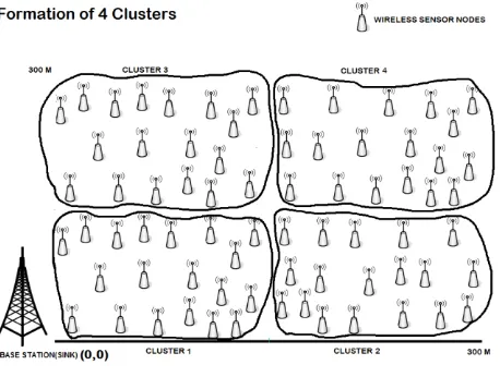
[image:2.595.314.543.275.448.2] Energy Consumption is based on First Order Radio model [6].
Fig 2: Formation of 4 Clusters in Proposed Technique
7.
BASIC PARAMETERS FOR
[image:2.595.309.542.509.754.2]SIMULATION AND THEIR INITIAL
VALUES
Table 1. Basic parameters for simulation
SN Parameter Name Unit Parameter
Value
1
Total number of nodes NOS 2502
Nodes Range NOS 200-3503
Geographical Area MTR 300 x 3004
Initial energy of each node (Ein)JOULES 200
5
Packet size (k) BYTES 1006
Energy circuitry cost at transmission and reception of a bit of data (Eelec )NJ/BIT 50
7
Amplifier coefficient(Eamp)PJ/BIT/M4 100
8
Coordinate of base station8.
PERFORMANCE ANALYSIS OF
EEHRP
To evaluate the performance of our algorithm EEHRP we simulated EEHRP using 250 nodes in a geographical of 300x300 square mtr. We divided the whole area into four equal clusters see Figure 2. Formation of cluster is done according following criterion.
8.1 Cluster Formation Criterion
For first cluster (see Figure 3), range lies between X coordinate=0-150 Y coordinate=0-150
Fig 3: First Cluster
For Second cluster (see Figure 4), range lies between X coordinate=151-300
Y coordinate=0-150
Fig 4: Second Cluster
For Third cluster (see Figure 5), range lies between X coordinate=0-150
Y coordinate=151-300
Fig 5: Third Cluster
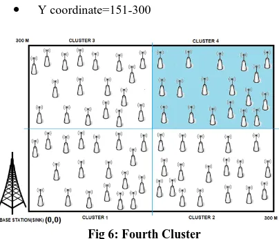
For Fourth cluster (see Figure 6), range lies between X coordinate=151-300
Y coordinate=151-300
Fig 6: Fourth Cluster
Deployment of sensor nodes is random within geographical area. We provided random x and y coordinates to each sensor node within range of 0 to 300. According to their coordinates each node belongs to a cluster i.e. 1, 2, 3 or 4. We simulated the algorithm steps for 400 rounds.
[image:3.595.318.520.72.245.2]In Figure 7 the whole network is divided into three clusters. Nodes within a cluster having same symbol but differ than nodes in other cluster.
Fig 7: Second level hierarchical formation with differentiated colors indicating difference in three clusters
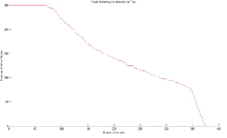
[image:3.595.314.541.357.485.2]15 Fig 9: Nodes energy residue in second level hierarchical
technique after 400 rounds simulation (When Number of cluster=3)
In Figure 10 the whole network is divided into four clusters. Nodes within a cluster having same symbol but differ than nodes in other cluster.
[image:4.595.316.537.76.209.2]Fig 10: Second level hierarchical formation with differentiated colors indicating difference in four clusters
[image:4.595.310.540.77.400.2]Fig 11: Network Life Time Graph for Second level hierarchical technique (When Number of cluster=4)
Fig 12: Nodes energy residue in second level hierarchical technique after 400 rounds simulation (When Number of
[image:4.595.313.542.257.399.2]cluster=4)
Fig 13: Comparison of Network Life Time for different Level of Hierarchy (Proposed NOC=4)
8.2 SIMULATION RESULTS
Table 2. Simulation Result Table Showing Network Life Time (M is number of clusters)
NUMBER OF NODES
NETWORK LIFE TIME (IN ROUNDS WHEN ALL
NODES DIE)
M=1 M=2 M=3 M=4
200 110 205 305 360
250 120 190 325 375
300 130 185 335 335
350 140 185 365 365
Table 3. Simulation Result Table Showing Mean Residual Energy of sensor nodes (M is number of clusters)
NUMBER OF NODES
MEAN RESIDUAL ENERGY
M=1 M=2 M=3 M=4
200 10 19 52 73
250 10 11 50 56
300 10 8 56 65
[image:4.595.57.289.306.437.2] [image:4.595.308.536.477.599.2] [image:4.595.58.288.484.624.2]9.
CONCLUSION
Proposed protocol in this paper is proved by evaluating the residual energy in each node for a particular round of simulation. The results in Table 2 and Table 3 show that the mean residual energy value of all the sensor nodes and Network lifetime of our proposed method is higher than the non hierarchical method which is a further indication of an improved network lifetime when our proposed technique is being implemented. Our Result is also better than second level hierarchical technique in which cluster formation were three.
10.
REFERENCES
[1] D.J. Pottie and W.J. Kaiser, “Wireless integrated network sensors”, Communication of the ACM, Vol. 43, No 5, pp 51-58, May 2000.
[2] Network Structure and Topology based Routing Techniques in Wireless Sensor Network- A survey Published in International Journal of Computer Applications (0975 – 8887) Volume 74– No.12, July 2013. [3] Subhadra Shaw (Bose) ,Energy-Efficient Routing Protocol in Wireless Sensor Network , International Journal of Scientific & Engineering Research Volume 2, Issue 12, December-2011.
[4] Subhadra Shaw (Bose), Energy-Efficient Routing Protocol in Wireless Sensor Network, International Journal of Scientific & Engineering Research Volume 2, Issue 12, December-2011.
[5] Shamsad Parvin and Muhammad Sajjadur Rahim, Routing Protocols for Wireless Sensor Networks: A Comparative Study, International Conference on Electronics, Computer and Communication (ICECC 2008) University of Rajshahi, Bangladesh.
[6] Heinzelman W, Chandrakasan A, Balakrishnan H. Energy-efficient communication protocol for wireless microsensor networks. Proceedings of the 33rd International Conference on System Science (HICSS’00), Hawaii, U.S.A., January 2000.
[7] I.F. Akyildiz et al., Wireless sensor networks: a survey, Computer Networks 38 (4) (2002) 393–422.
[8] J. N. Al-Karaki and A. E. Kamal, “Routing Techniques in Wireless Sensor Networks: A Survey”, IEEE Wireless Communications Magazine, vol. 11, no. 6, pp. 6-28, December, 2004.
[9] W. Heinzelman, J. Kulik, H. Balakrishnan, Adaptive protocols for information dissemination in wireless sensor networks in Proceedings of the 5th Annual ACM/IEEE International Conference on Mobile Computing and Networking (MobiCom_99), Seattle, WA, August 1999. [10]R. Alasem, A. Reda, and M. Mansour, “Location Based
Energy- Efficient Reliable Routing Protocol for Wireless Sensor Networks”, Recent Researches in Communications, Automation, Signal processing, Nanotechnology, Astronomy and Nuclear Physics, WSEAS Press, Cambridge, UK, 2011, ISBN: 978-960-474-276-9. [11]V. Rodoplu, T.H. Ming, Minimum energy mobile wireless
networks, IEEE Journal of Selected Areas in Communications 17 (8) (1999) 1333–1344.