http://dx.doi.org/10.4236/jep.2014.56055
Stochastic Approach on Forest Fire Spatial
Distribution from Forest Accessibility in
Forest Management Units, South
Kalimantan Province, Indonesia
Beni Raharjo, Nobukazu NakagoshiGraduate School for International Development and Cooperation (IDEC), Hiroshima University, Hiroshima, Japan Email: beni.raharjo@gmail.com
Received 24 February 2014; revised 25 March 2014; accepted 21 April 2014
Copyright © 2014 by authors and Scientific Research Publishing Inc.
This work is licensed under the Creative Commons Attribution International License (CC BY). http://creativecommons.org/licenses/by/4.0/
Abstract
This study explores stochastic approach to analyzing the forest fire spatial distribution from forest accessibility using 2-parameters Weibull distribution model. MODIS firespot data, as a proxy for forest fire location, from 2001 to 2012 was analyzed by correlating its spatial distribution with the distance from settlement and road/lake in 11 Forest Management Units (FMUs) in South Kali-mantan Province, Indonesia. The distribution parameters for 11 FMUs are αs = 5.45; βs = 1.42 for the distance from settlement and αrl = 0.87; βrl = 0.86 for the distance from road/lake. The forest fire spatial distribution equations are therefore
( )
(
)
s
F x = −1 exp − x 5.451.42 from settlement
and
( )
(
)
rl
F x = −1 exp − x 0.87 0.86 from road/lake, where x is the distance (km) from either settle- ment or road/lake. Further, a correlation was found between forest accessibility conditions and forest fire spatial distribution. The α- and β-parameters correlate to number of settlement (NS) and road intensity (RI) by αs=5.103−57.248⋅NS (with R2 = 0.77; Fsig = 0.01); βs =1.476+0.063⋅RI (with R2 = 0.65; Fsig = 0.03) for firespot spatial distribution from settlement and
rl =1.617−0.12⋅RI
α (with R2 = 0.57; Fsig = 0.01);
rl =1.015−0.015⋅RI
β (R2 = 0.33; Fsig = 0.07) for firespot spatial distribution from road/lake. The stochastic approach using 2-parameters Weibull distribution model has a reliable and practical application on assessing forest fire spatial distribution from forest accessibility.
Keywords
1. Introduction
The effect of the anthropogenic factor on forest fire is obvious. It has been reported that forest fire is rather anthropogenic phenomena [1]-[4]. More quantitatively Adinugroho, Suryadiputra, Saharjo and Siboro [5] stated that 99% of Indonesian fire is human triggered. The similar finding was revealed by Tomich, et al. [6] that In-donesian forest fire occurs because it is the main tool for land preparation in shifting cultivation, transmigration, and timber and oil plantation. Study on anthropogenic factors on forest fire distribution is based on the assump-tion that the main fire hazard source is human and the probability of the fire is higher where the accessibility is easier [7]. Therefore, the Indonesian forest fire spatial distribution is related to forest accessibility.
The forest fire risk study has been done through overlaying various potential influencing factors such as slope, altitude, proximity to road/settlement, vegetation cover [8], stand age, species’ composition, and crown closure
[9]. Accessibility (proximity to road/settlement) has been accommodated arbitrarily. Erten, Kurgun and Musaoglu [10], for example, classified the distance from settlement into very high (0 - 1000 m), high (1000 - 2000 m), medium (2000 - 3000 m) and low (>3000 m) fire risk classes. Meanwhile, Darmawan, Aniya and Tsuyuki [11], buffered the forest from the road by high (0 - 250 m), moderate (250 - 500 m), low (500 - 1000 m), and none (>1000 m) fire risk classes in a forest fire study, in Indonesia. A more simple classification was used by Badarinath, Madhavilatha, Chand and Murthy [12] in developing a Human Risk Index for modeling potential forest fire danger using 1 kilometer from roads, 1.5 kilometers from settlements and 100 meters from the river as the class limits. That arbitrary classification has been widely used due to unavailability of the quantitative classi-fication technique on forest fire spatial distribution from forest accessibility. However, since the accurate and consistent fire probability classes are essential for efficient forest fire management [13], a more quantitative method is required. Therefore, better approaches need to be introduced to quantify the forest fire spatial distribu-tion from forest accessibility.
Stochastic approaches have been widely used in forest fire studies. Finey, et al. [14] studied a simulation on probabilistic fire assessment on the continental scale. Jiang, Zhuang and Mandallaz [15] used Poisson distribu-tion to modeled large fire frequency and burned area in Canada. Grissino-Mayer [16] also studied forest fire in-terval in United State using Weibull Model. A study on forest fire growth model was conducted by Boychuk, et
al. [17] using a stochastic approach. Forest fire is, therefore, considered as stochastic phenomena [18] and
sto-chastic approach also has a possible application to analyze the forest fire spatial distribution.
The objective of this study is to model and explore the application of stochastic approach on forest fire spatial distribution from forest accessibility features, i.e. settlement, road and lake using 2-parameters Weibull distribu-tion model.
2. Methods
MODIS firespot data from 2001 to 2012 was used as the proxy of the forest fire location. The distances of fire-spot from the closest settlement and road/lake were calculated, ranked and plotted. Distribution fittings were run to find the Weibull distribution α- and β-parameters. Then, validations on the reliability of the estimated distri-butions using goodness-of-fit test were performed on the resultant distridistri-butions. Resultant parameters were cor-related with possible explanatory variables using multiple linear regression analyses.
2.1. Study Site
South Kalimantan Province is located in the south-east part of Borneo Island. It lays from 114˚21'E to 116˚33'E and from 1˚17'S to 4˚18'S. With the land size about 3.75 million hectares, it has forest area about 48% or 1.8 million hectares [19]. It has been designed that all forests are managed under eleven Forest Management Units (FMUs) as can be seen inFigure 1. All FMUs were used as the study sites of this study. However, for validation and simulation purpose, only FMU XI was selected.
2.2. Data
The study used two data types, i.e. forest firespot locations and forest accessibility features. MODIS firespots data, as a proxy for forest fire location, is the near real-time position of active fires that are derived from stan-dard MODIS MOD14/MYD14 Fire and Thermal Anomalies product. It was acquired from Fire Information for Re- source Management System [20]. The numbers of 5,678 firespot within FMUs from 2002 to 2012 were recorded
Figure 1. Eleven forest management units in South Kali-mantan province, Indonesia.
Table 1. Number of firespot in eleven FMUs from 2001 to 2012.
FMU Year Total
2001 2002 2003 2004 2005 2006 2007 2008 2009 2010 2011 2012
I 14 169 84 138 56 158 33 6 104 3 57 26 848
II 1 189 55 96 54 121 14 6 74 1 30 61 702
III 129 23 43 26 192 13 8 103 1 37 53 628
IV 1 65 11 29 7 39 5 49 18 17 241
V 3 26 4 26 12 37 12 11 32 1 4 8 176
VI 10 160 52 146 37 224 24 6 71 2 35 34 801
VII 15 102 81 149 51 150 13 4 147 6 75 44 837
VIII 19 11 26 7 30 10 4 9 4 7 127
IX 31 62 35 37 26 62 20 1 45 2 45 15 381
X 6 37 5 10 6 20 5 5 33 1 20 5 153
XI 38 119 88 102 57 168 30 7 91 4 47 33 784
[image:3.595.92.539.499.724.2]of scale 1:50,000 issued in 2007 by Indonesian National Mapping and Survey Coordination Agency (BAKOSURTANAL). Additional data of FMUs boundaries were obtained from Forestry Service of South Ka-limantan Province. All spatial data was processed in digital format using WGS84 datum and UTM Zone 50S projection.
2.3. Distribution Parameters Estimation
Two parameter estimations were performed in firespot spatial distribution from settlement and firespot spatial distribution from road/lake. Euclidean distances from the closest settlement and closest road/lake were calculated for each firespot. The Empirical Distribution Function (EDF) was estimated on ascending sorted distance data using a median formula [21] of F xˆ
( ) (
i = −i 0.3) (
n+0.4)
where F xˆ( )
i is the cumulative empiricalprobabil-ity, i is the rank of the i-th sorted firespot distance and n is the total number of firespot. The resultant EDF has possible value within 0 - 1 range.
The 2-parameters Weibull distribution model was selected because its elasticity which can mimics many dis-tributions such as Normal, Lognormal, Exponential and Rayleigh disdis-tributions [21]. The distribution also has ability to fit data from various field such as life, weather, economics, administration, hydrology, biology or en-gineering science [22]. The Weibull Probability Density Function (PDF) is the distribution for continuous va-riables. Bedient and Huber [23] suggested using Cumulative Distribution Function (CDF) which is the integral form of the PDF. The PDF of 2-parameters Weibull Distribution can be written as
( ) (
)(
)
1(
(
)
)
exp
f x = β α xα β− − xα β (1)
with its corresponding CDF of
( )
1 exp(
(
)
)
F x = − − xα β (2)
where
x : distance from either settlement or lake/road (x ≥ 0) (km)
α : scale parameter (α ≥ 0)
β : shape parameter (β ≥ 0)
To estimates the distribution parameters from sample data, some parameter estimation methods have been developed. This study uses Maximum Likelihood Estimator (MLE) to estimate α- and β-parameters because it is a robust and converge estimation for the Weibull distribution [24]. Moreover, the software to perform the MLE is available in the open source R Statistical Software [25] with additional fitdistrplus, survival, splines and re-shape 2 packages.
The likelihood function assumes that there is an unknown parameter (θ) in the PDF (Equation (1)) which is then written as f x
( )
,θ . Thus, the likelihood function of the random sample is the joint density of x x1, 2,,xnand the unknown parameter (θ) [26] as follow.
( )
1 , i n x iL f xθ
=
=
∏
(3)Using the Equation (1) and Equation (3), the likelihood function is then written as
(
)
(
)(
)
1(
(
)
)
1
1
, , , , exp
n
n
i
L x x α β β α xα β− xα β
=
=
∏
− (4)
The MLE of θ is the value of θ that maximize the value of the likelihood function (L). By taking logarithm of Equation (4) and then differentiated it respect to β and α and equating to zero, the Equations (5) and (6) were generated.
1 1
ln 1
ln ln 0
n n
i i i
i i
L n
x xβ x
β β = α =
∂
= + − =
∂
∑
∑
(5)2 1 ln 1 0 n i i L n xα
α α α =
∂ −
= + =
By eliminating α in the Equations (5) and (6), the Equation (7) was used to estimate β.
1 1 1
1 1
ln ln 0
n n n
i i i i
i i i
x x x x
n
β β
β
= = =
− − =
∑
∑
∑
(7)The iterative calculation was applied to solve the Equation (7). If β-parameter has been estimated from the iteration, the α-parameter can be solved by the Equation (8).
1
n
i i
xβ n α
=
=
∑
(8)2.4. Goodness-Of-Fit Test
This study used Kolmogorov-Smirnov Test (K-S test) to measure the discrepancy between the resultant distribu-tion (Weibull CDF) and the firespot data distribudistribu-tion (EDF). A significance level of ρ = 0.01 was used in the test. If the resultant probability of K-S test (K-S ρ) was bigger than 0.01, then the resultant distribution fit the data. K-S test calculated the maximum value of the difference (D) of EDF and CDF [22] which can be shown in the following formula.
(
)
sup EDF CDF
D= − (9)
where
D : The maximum different between CDF and EDF EDF : Empirical Distribution Function
CDF : Cumulative Distribution Function
2.5. Probability Classification
[image:5.595.170.456.575.705.2]Probability classification of forest fire spatial distribution was performed. The numbers of four classes (Class I – IV) were derived from the CDF of firespot in all fit distributions by using equal proportions method. Thus, the fire probability was divided by 3 quartiles, i.e. Q1 (F(x)= 0.25), Q2 (F(x) = 0.5) and Q3 (F(x)= 0.75) as shown in
Figure 2. The resultant four classes were compared with a number of firespot falls within each class to validate
the result. The Sultan Adam Forest Park (FMU XI) was selected for validation.
2.6. Multiple Linear Regression Analysis
In order to find a correlation between resultant firespot spatial distributions and accessibility conditions inTable 2, multiple regression analyses were performed using backward elimination method by the following model.
(
)
; ; ; , , ,
s s rl rl f A NS PS RI
α β α β = (10)
where
s
α = scale parameter (from settlement)
s
β = shape parameter (from settlement)
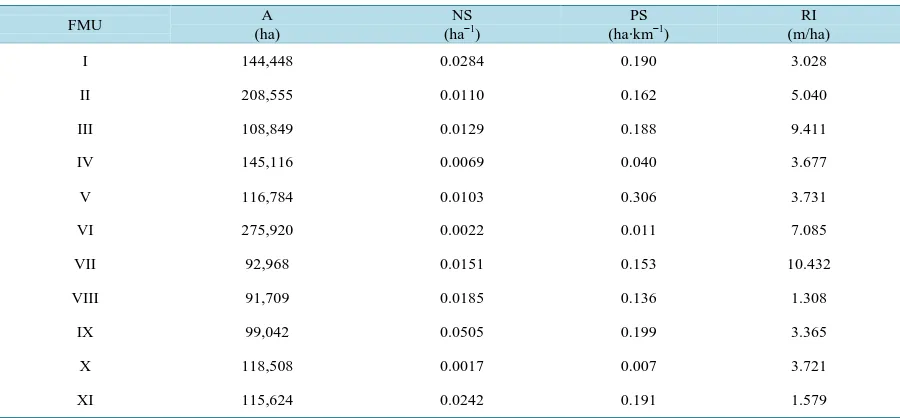
Table 2. Potential explanatory variables of forest accessibility conditions for α- and β-parameters.
FMU A
(ha)
NS (ha−1)
PS
(ha∙km−1) (m/ha) RI
I 144,448 0.0284 0.190 3.028
II 208,555 0.0110 0.162 5.040
III 108,849 0.0129 0.188 9.411
IV 145,116 0.0069 0.040 3.677
V 116,784 0.0103 0.306 3.731
VI 275,920 0.0022 0.011 7.085
VII 92,968 0.0151 0.153 10.432
VIII 91,709 0.0185 0.136 1.308
IX 99,042 0.0505 0.199 3.365
X 118,508 0.0017 0.007 3.721
XI 115,624 0.0242 0.191 1.579
A = size of the forest; NS = number of settlement; PS = proportion of settlement size; RI = road intensity.
rl
α = scale parameter (from road/lake)
rl
β = shape parameter (from road/lake) A = size of the forest / FMU (ha) NS = number of settlement (km−2)
PS = proportion of settlement size (ha∙km−2) RI = road intensity (m∙ha−1)
3. Results
Distribution fitting was successfully performed in both firespot spatial distribution from the settlement and road/lake. Sets of α- and β-parameters for all eleven FMUs and each FMU were successfully estimated. The plots of histograms and estimated firespot spatial distributions from the settlement are shown inFigure 3, while those from road/lake are shown inFigure 4.
The estimated parameters of firespot spatial distribution from the settlement in all 11 FMUs were αs = 5.45
and βs = 1.42. However, parameters vary in each FMU within the range of αs = 2.29 – 5.6 and βs = 1.23 – 2.22.
While the estimated parameters from road/lake in all 11 FMUs were αrl = 0.87 and βrl = 0.86 within the range of
αrl = 0.5 – 1.87 and βrl = 0.81 – 1.03. The list of estimated distribution parameters is presented in Table 3.
The discrepancies between estimated distribution and the firespot data distribution were tested by K-S test. It is observed that, from the settlement, there are four distributions of FMU III, FMU IV, FMU VI and FMU X which did not pass the K-S test. On the other hand, all firespot distributions from road/lake fit the firespot data in All FMUs (Table3).
Since the firespot spatial distributions were estimated in probabilistic models, quartiles and mode of those distributions were easily derived from the model as shown inTable 4. For all FMUs, the first quartile (Qs1) of
2.26 km, the second quartile (Qs2) of 4.21 km and the third quartile (Qs3) of 6.85 km were derived from firespot
distribution from the settlement. Meanwhile, the first quartile (Qrl1) of 0.2 km, the second quartile/median (Qrl2)
of 0.57 km and the third quartile (Qrl3) of 1.27 km were derived from firespot distribution from road/lake. The
modes Mo which represent the highest probability of firespot were derived at Mos = 2.31 km from settlement
(ranges 1.04 - 3.77 km). Meanwhile, for the firespot distribution from road/lake, modes can be derived only in FMU I, FMU IX and FMU X with the range of 0.04 - 0.05 km.
Figure 3. Histograms and estimated firespot spatial distribution from settlement in FMUs.
pected proportion of 25% in each class.
Multiple linear regression analysis regressed firespot spatial distribution (distribution parameters) and forest accessibility conditions. The selected linear models are αs=5.103 57.248− ⋅NS (with R2 = 0.77; Fsig = 0.01) and βs =1.476 0.063+ ⋅RI (with R2 = 0.65; Fsig = 0.03) for the firespot distribution from settlement. While,
1.617 0.12
rl RI
α = − ⋅ (with R2 = 0.57; Fsig = 0.01) and βrl =1.015 0.015− ⋅RI (with R2 = 0.33; Fsig = 0.07) were selected for the firespot distribution from road/lake (Table 5).
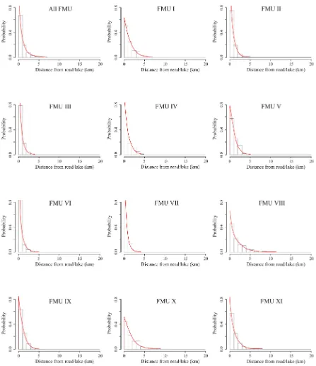
Figure 4. Histograms and estimated firespot spatial distribution from road/lake in FMUs.
shows that the increase of NS by 100% shifts the firespot distribution closer to settlement, while, the increase of RI by 400% shifts the firespot distribution away from the settlement and also closer to road/lake (Figure 6).
4. Discussion
Figure 5. Map of firespot distribution in FMU XI overlaid with firespot spatial probability classes (a) from set-tlement and (b) from road/lake.
Figure 6. Simulations on the increase of NS and RI (in FMU XI) on firespot distribution (a) from settlement and (b) from road/lake.
Table 3. Estimated distribution parameters and K-S test Results.
FMU From settlement From road/lake
αs βs K-S ρ αrl βrl K-S ρ
I 3.64 1.76 0.425 1.43 1.03 0.212
II 4.41 1.55 0.037 0.72 0.95 0.916
III 5.60 1.89 0.000* 0.57 0.91 0.036
IV 4.12 1.23 0.000* 0.93 0.99 0.136
V 4.20 1.55 0.111 0.93 0.99 0.136
VI 5.09 1.72 0.000* 0.57 0.81 0.587
VII 4.93 2.22 0.264 0.50 0.83 0.044
VIII 4.24 1.58 0.243 1.79 0.89 0.677
IX 2.29 1.83 0.156 0.94 1.03 0.957
X 3.71 1.42 0.007* 1.87 1.02 0.659
XI 3.02 1.62 0.643 1.23 0.93 0.887
All FMU 5.45 1.42 0.016 0.87 0.86 0.215
[image:9.595.89.538.504.709.2]Table 4. Quartiles and modes of estimated firespot spatial distribution.
FMU
From settlement From road/lake
Qs1 (km) Qs2 (km) Qs3 (km) Mos (km) Qrl1 (km) Qrl2 (km) Qrl3
(km) Mos (km)
I 1.80 2.96 4.39 2.26 0.43 1.00 1.96 0.05
II 1.98 3.48 5.44 2.27 0.19 0.49 1.01 -
III 2.89 4.61 6.65 3.76 0.15 0.38 0.81 -
IV 1.49 3.05 5.38 1.04 0.26 0.64 1.30 -
V 1.88 3.32 5.18 2.16 0.26 0.64 1.30 -
VI 2.47 4.11 6.15 3.07 0.12 0.36 0.85 -
VII 2.81 4.18 5.71 3.77 0.11 0.32 0.73 -
VIII 1.93 3.36 5.21 2.25 0.44 1.19 2.59 -
IX 1.16 1.87 2.74 1.49 0.28 0.66 1.28 0.04
X 1.54 2.86 4.67 1.56 0.55 1.31 2.58 0.04
XI 1.41 2.41 3.70 1.68 0.32 0.83 1.75 -
All FMU 2.26 4.21 6.85 2.31 0.20 0.57 1.27 -
Q1 = first quartile; Q2 = second quartile (median); Q3 = third quartile; and Mo = modes (peak).
Table 5. The multiple regression analysis result between α- and β-parameters and forest accessibility conditions. Distribution
parameters
Explanatory
Variables R
2 Fsig Models
αs NS 0.77 0.01 αs=5.103 57.248− ⋅NS
βs RI 0.65 0.03 βs=1.476+0.063⋅RI
αrl RI 0.57 0.01 αrl=1.617−0.12⋅RI
βrl RI 0.33 0.07 βrl=1.015−0.015⋅RI
αs = scale parameter for settlement; βs = shape parameter for settlement; αrl= scale parameter for road/lake; βrl = shape parameter for road/lake; NS =
number of settlement (sett.km−2); RI = road density (m∙ha−1).
2-parameters Weibull distribution.
The selection of the MODIS firespot data as a proxy of forest fire location has some limitations. The firespot points are not truly the locations of fires. The 1 kilometer spatial resolution of the MODIS images [27] can be considered as low spatial resolution image. Also, the real forest fire in the field never exists in point, but rather in the area. However, sensing the forest fire by the satellite images has enormous advantages from early fire de-tection capability [28], very high temporal resolution and near real time data availability. In addition, this study tried to assess the spatial forest fire distribution in a quite large study area. It is, therefore, considerably appro-priate to use MODIS firespot to represent forest fire location in this study.
It was seen that in 4 FMUs (FMU III, FMU IV, FMU VI and FMU X) the estimated spatial distributions of firespot from settlement did not fit the data (Table 3) because the K-S ρ values were lower than the defined 0.01 threshold. As can be seen inFigure 3, the estimated distributions in those FMUs have wide discrepancies from the histograms. It is visually observed the presence of multimodality of firespot distribution on those four FMUs can be the reason for unfit Weibull distribution.
[image:10.595.88.534.380.470.2]probability of forest fire. On the other hand, in forest fire spatial distribution from road/lake, the mode is right on the road or edge of the lake. Hence, the forest fire probability classification can be started from the road or the lake.
The α-parameter determines the span of the Weibull distribution. It also shows the characteristic of life in which about 63.21% [22] of the forest fire occurs before x = α. The α-parameter provides quick figure about the resultant distributions. In firespot distribution from the settlement, the characteristic of life for all FMUs is 5.45 (ranges 2.29 - 5.45 km) from settlement. While, in firespot distribution from road/lake, the characteristic of life for all FMUs is 0.87 (ranges 0.5 - 1.87 km). Hence, forest fire distribution is more concentrated around road/lake instead of around settlement.
The β-parameters determine the shape of the distribution and, therefore, determine the flexibility of the dis-tribution. If β = 1 the distribution is identical to the exponential distribution, If β = 2 the distribution is identical to the Rayleigh distribution, and if β is between 3 and 4 the distribution is close to normal distribution [22]. In firespot distribution from settlement, the β-parameters is 1.42 (ranges 1.23 - 2.22), while for those from road/lake the β-parameters is 0.86 (ranges 0.81 - 1.03). Forest fire spatial distribution from road/lake has mode around the road or edge of the lake because β is close to 1. Meanwhile, the forest fire spatial distributions from settlement show the unimodal shape with mode noticeably far (ranges 1.04 - 3.77 km) from settlement.
Further, as an additional analysis to correlate the behavior of distribution (parameters) with explanatory va-riables, the regression analyses were used. The regression models inTable 5 are beneficial to predict the effect of the change of NS and RI on the forest fire spatial distribution from accessibility. As shown inFigure 6, the increase of NS shifts the firespot distribution closer to settlement. Higher NS within forest may reduce the range for human activities within the forest. While, the increase of RI shifts firespot distribution is farther from settle-ment and closer to road/lake. The RI affects not only the firespot spatial distribution from road/lake, but also from settlement. The road/lake extends the forest fire spatial distribution farther from settlement.
This study provides evidence that forest fire is more anthropogenic rather than naturally occurs. First, the for-est fire probability is relatively low in the area closer to settlement and increase along the distance until it reach-es the maximum probability. It shows that human prefers to minimize the forreach-est fire in the area closer to settle-ment. Second, the probability of forest fire decreases along the increase of the distance from the settlement after it reaches the maximum probability. The distance barriers the forest fire to ignite deeper into the forest due to human limitation to travel from settlement to deeper forest. Third, the highest fire probability is right on the road or edge of the lake. Travelling farther from road/lake increase the cost and certainly not preferred.
The stochastic approach provides a more quantitative method compare to arbitrary approach for assessing the effect of the accessibility on the forest fire spatial distribution. This approach also has an advantage due to the nature of the forest fires are stochastic [18]. The approach also gives practical benefit for forest fire management due to its flexible application for probability classification.
4. Conclusion
The stochastic approach has reliable and practical applications on assessing forest fire spatial distribution from forest accessibility. The study proposes the cumulative forest fire spatial distribution models of
( )
(
)
1.421 exp 5.45
F x = − − x from settlement and F x
( )
= −1 exp−(
x 0.87)
0.86 from road/lake. However, the distributions vary among the forests and, therefore, forest fire spatial distribution can be estimated in each forest by αs=5.105 57.248− ⋅NS; βs =1.476 0.063+ ⋅RI from settlement and αrl =1.617 0.12− ⋅RI;1.015 0.015
rl RI
β = − ⋅ from road/lake.
Acknowledgements
The authors would like to thank to Monbukagakusho/MEXT scholarship for funding support. Authors also thank to FIRMS NASA and Forestry Service of South Kalimantan Province for providing valuable data and informa-tion.
References
[2] Martinez, J., Vega-Garcia, C. and Chuvieco, E. (2009) Human-Caused Wildfire Risk Rating for Preventing Planning in Spain. Journal of Environmental Management, 90, 12.
[3] Kalabokidis, K., Xanthopoulos, G., Moore, P., Caballero, D., Kallos, G., Llorens, J., Roussou, O. and Vasilakos, C. (2012) Decision Support System for Forest Fire Protection in the Euro-Mediterranean Region. European Journal of Forest Research, 131, 597-608. http://dx.doi.org/10.1007/s10342-011-0534-0
[4] Haryati, E. and Nakagoshi, N. (2013) Post-Fire Succession at Forest Vegetation in Giam Siak Kecil Wildlife Reserve, Riau, Indonesia. Hikobia Journal, 16, 335-349.
[5] Adinugroho, W.C., Suryadiputra, I.N.N., Saharjo, B.H. and Siboro, L. (2005) Manual for the Control of Fire in Peat-lands and Peatland Forest. In: Book Manual for the Control of Fire in Peatlands and Peatland Forest, Wetlands Inter-national-Indonesia Programme and Wildlife Habitat Canada, Bogor.
[6] Tomich, T., Fagi, A., Foresta, H.D., Michon, G., Murdiyarso, D., Stolle, F. and Noordwijk, M.V. (1998) Indonesia’s Fires: Smoke as a Problem, Smoke as a Symptom. Agroforestry Today, 10, 4-7.
[7] Murdiyarso, D., Widodo, M. and Suyamto, D. (2002) Fire Risks in Forest Carbon Projects in Indonesia. Science in China Series C-Life Sciences, 45, 65-71.
[8] Hernandez-Leal, P.A., Arbelo, M. and Gonzalez-Calvo, A. (2006) Fire Risk Assessment Using Satellite Data. Natural Hazards and Oceanographic Processes from Satellite Data, 37, 741-746.
[9] Thompson, W.A., Vertinsky, I., Schreier, H. and Blackwell, B.A. (2000) Using Forest Fire Hazard Modelling in Mul-tiple Use Forest Management Planning. Forest Ecology and Management, 134, 163-176.
http://dx.doi.org/10.1016/S0378-1127(99)00255-8
[10] Erten, E., Kurgun, V. and Musaoglu, N. (2004) Forest Fire Risk Zone Mapping from Satellite Imagery and Gis a Case Study. Proceedings ISPRS Proceeding, 33-39.
[11] Darmawan, M., Aniya, M. and Tsuyuki, S. (2001) Forest Fire Hazard Model Using Remote Sensing and Geographic Information Systems: Toward Understanding of Land and Forest Degradation in Lowland Areas of East Kalimantan, Indonesia. In: Book Forest Fire Hazard Model Using Remote Sensing and Geographic Information Systems: Toward Understanding of Land and Forest Degradation in Lowland Areas of East Kalimantan, Indonesia, Centre for Remote Imaging, Sensing and Processing (CRISP), National University of Singapore, Singapore.
[12] Badarinath, K.V.S., Madhavilatha, K., Chand, T.R.K. and Murthy, M.S.R. (2004) Modeling Potential Forest Fire Dan-ger Using Modis Data. Journal of Indian Society of Remote Sensing, 32, 343-350.
http://dx.doi.org/10.1007/BF03030859
[13] Seol, A., Lee, B. and Chung, J. (2012) Analysis of the Seasonal Characteristics of Forest Fires in South Korea Using the Multivariate Analysis Approach. Journal of Forest Research, 17, 45-50.
http://dx.doi.org/10.1007/s10310-011-0263-8
[14] Finey, M.A., McHugh, C.W., Grenfell, I.C., Riley, K.L. and Short, K.C. (2011) A Simulation of Probabilistic Wildfire Risk Components for the Continental United States. Stochastic Environmental Research and Risk Assessment, 25, 973- 1000.
[15] Jiang, Y.Y., Zhuang, Q.L. and Mandallaz, D. (2012) Modeling Large Fire Frequency and Burned Area in Canadian Terrestrial Ecosystems with Poisson Models. Environmental Modeling & Assessment, 17, 483-493.
http://dx.doi.org/10.1007/s10666-012-9307-5
[16] Grissino-Mayer, H.D. (1999) Modeling Fire Interval Data from the American Southwest with the Weibull Distribution.
International Journal of Wildland Fire, 9, 37-50.
[17] Boychuk, D., Braun, W.J., Kulperger, R.J., Krougly, Z.L. and Stanford, D.A. (2009) A Stochastic Forest Fire Growth Model. Environmental and Ecological Statistics, 16, 133-151. http://dx.doi.org/10.1007/s10651-007-0079-z
[18] Gilless, J.K. and Fried, J.S. (1998) Stochastic Representation of Fire Behavior in a Wildland Fire Protection Planning Model for California. Forest Science, 45, 492-499.
[19] MoF (2009) Ministry of Forstry Decree No Sk.435/Menhut-Ii/2009 on Establishment of Forest Area in South Kali-mantan Province. Book Ministry of Forstry Decree No. Sk.435/Menhut-Ii/2009 on Establishment of Forest Area in South Kalimantan Province, Ministry of Forestry, Jakarta.
[20] Firms, N. (2012) Modis Hotspot/Active Fire Detections. Book Modis Hotspot/Active Fire Detections.
[21] Murthy, D.N.P., Xie, M. and Jiang, R. (2004) Weibull Models. Wiley Interscience, New Jersey.
[22] Rinne, H. (2009) The Weibull Distribution: A Handbook. CRC Press, Boca Raton.
[23] Bedient, P.B. and Huber, W.C. (1992) Hydrology and Floodplain Analysis. Addison-Wesley, Reading, Mass.
[24] Gove, J.H. (2003) Moment and Maximum Likelihood Estimators for Weibull Distributions under Length- and Area- Biased Sampling. Environmental and Ecological Statistics, 10, 455-467.
[25] Team, R.D.C. (2011) R: A Language and Environment for Statistical Computing. In: Book R: A Language and Envi-ronment for Statistical Computing, R Foundation for Statistical Computing, Vienna.
[26] Bhattacharya, P. (2010) A Study on Weibull Distribution for Estimating the Parameters. Journal of Applied Quantita-tive Methods, 5, 8.
[27] Giglio, L. (2010) Modis Collection 5 Active Fire Product User’s Guide Version 2.4. In: Book Modis Collection 5 Ac-tive Fire Product User’s Guide Version 2.4, University of Maryland.