Measuring Processor Frequency for Load Stability in
Multi-Core MIMD Architecture
Hari Nandan
M.Tech(IT)
GNDEC, Ludhiana
Amanpreet Singh Brar
Associate Prof. & Head GNDEC, Ludhiana
Ankit Arora
Assistant Professor. LLRIET, Moga
ABSTRACT
Parallelism, a massive achievement in the field of processor architecture leading towards increased speed up by incorporating data as well as computation intensive work. Parallel architectural components interconnected with major consideration as communication among coupled hardware in order to stabilize workload distribution and management. Workload distribution with load stability fundamentally a tricky aspect of parallel distribution. Static policies covers load factors which are pre-determined before actually distribution takes place. Dynamic load stability and distribution periodically measures the load for each and every processor in heterogenic parallel processor systems.. Development of heterogenic multiprocessor machines with dynamic load stability matrices or measurements incorporates vast amount of efforts and covers varied amount of configuration factors on the behalf of the underlying communication architecture. So much of the processor’s efforts may lose for load stabilization, which may be controlled by improved dynamic load stability techniques and theories. In this research, the major aspect of development is to measure processor efficiency by analyzing frequency speed along with current processor load, only then the distribution takes place. Measuring cycle speed (i.e. no. of cycle per second elapsed) in terms of Hz, Mhz, Ghz is one of the measurement metric to analyze the processor efficiency. Further the research covers MIMD based core processor simulation version integrate frequency based distribution for load steadiness and control. Although, load consistency will not be completely managed with in any type of system. Load steadiness and uniformity will only be controlled up to some extent.
General Terms
Dynamic Job scheduling, Load Balancing and consistency, Processor Efficiency, Multi-Core MIMD Systems, Cycle Speed.
Keywords
Heterogenic Multi-Core Processor Simulation, Load steadiness, Workload Distribution, Time Sharing Environment, Frequency Cycle Speed Measurements.
1.
INTRODUCTION
Experimental research generally covers homogeneous processor interconnection structures, this is because the underlying platforms used for test scenarios provides such types of environment. Homogeneous structures generally covers redundant logic and parametric values which are common and fixed for each and every hardware linked. Simulation behind Heterogenic processor designs requires great deal of implementation work if structure covers scheduling as well as load balancing and other dynamic
constraints. One of the major bottlenecks among parallel execution is job scheduling which mostly covers time sharing and space sharing aspects of distribution [2][9]. Scheduling at operating system level covers global scheduling at upper level, which manages jobs that are firstly arranged in disk queue. At lower level processors local scheduling exists manages their own local ready queue management. Static aspects of scheduling cover factors such as capacity of memory buffers, no. of jobs scheduled, their arrivals etc. Dynamic scheduling on the other hand covers processor frequency speed, their periodic workload management and final job distribution after workload characterization. Further the research towards this field covers dynamic factor of workload analysis by estimating processor efficiency in terms of frequency measurement. Simulated version is developed to analyze the performance of heterogenic multi-core processors incorporating dual core and tri/quad core structures. Jobs are distributed among processors by estimating their cycle speed in terms of seconds by comparing their existing load and current incoming job workload. Job workload is considered as burst cycles arranged via random distribution mechanism in the incoming batch queue. Simulated log will be generated containing workload estimation of each and every processor core including overall workload estimation. Finally, the graphical results are produced to describe load stability and steadiness growth over different time barriers. Although different samples have been taken in analysis process which exhibit up to vast amount of extent the load will be balanced, distribution consistency will only be controlled, not completely fully balanced. Idea behind this research implementation is to understand the working of multi-core heterogenic architectures which are not generally available in today parallel machines Experimentation is possible only in simulation environment virtually designed to produce effects which may or may not be close to real results depending upon the logical configuration implementation and methodologies used.
2.
LITERATURE REVIEW
load balancing framework and run times software system for supporting the development of adaptive applications on distributed-memory parallel computers. The runtime system support a global namespace, transparent object migration, automatic message forwarding and routing, and automatic load balancing. Research towards distributed job processing with dynamic load balancing has been also described by P. Srinivasa Rao in a paper “Dynamic Load Balancing With Central Monitoring of Distributed Job Processing System” 2013, the detail covers Dynamic load balancing with a centralized monitoring capability. The purpose of using a centralized monitoring feature was based on the idea that the computation in a environment may be distributed, but the status of each task or job must be available at a central location for monitoring and better scheduling. This also allows better management of the jobs. The framework also addresses the inherent need for uniform load distribution by allowing the dispatcher to check against the status of the processors before a job is dispatched for processing.
3. OBJECTIVE
Objective is to simulate heterogenic Multi-Core processor architectures by measuring processor efficiency in terms of processor frequency speed along with present processor load and incoming workload distribution. The idea covers dynamic aspect for load steadiness and constancy during job scheduling in heterogenic environment. Each processors 1-cycle time will be calculated and remaining 1-cycles still to be processed will be measured along with new job workload cycles. The processor which consumes minimum amount of time will undertakes that particular job and in this way distribution takes place.
4.
WORKLOAD CHARACTERIZATION
Workload selection for simulation implementation is based upon random distribution. Front end long term queue will be build to carry virtual job description, which further covers process id, their time in terms of burst cycles requires. Such burst cycles are actually the no. of CPU cycles required to process by each job. Such data is arranged automatically during simulation execution. Input data covers such types of aspects, resultant output data will carry workload detail on processor cores described in terms of status log of the processors. The status log exhibits individual load of each processor core and finally the overall load of the processor, on basis of which overall workload distribution of job scheduling takes place. Other detail includes no. of jobs processed by each core, their pending workload status. The log will be maintained periodically behind database as well. This is required at different time barriers because collection of simulation results at differential time samples will actually justify the results. Below is the dummy sample of status log grid demonstrated in the fig-12. First attribute represents time barrier basis on which the periodic simulation results will be measured. Processor frequency describes the type of processor speed. Other parametric values describe the varying load of each of the processor core. The results collected after executing simulation no. of times and describes that the load steadiness is maintained up to very large extent, although not completely fully controlled but above 85% is controlled and consistent
.
Load estimator estimates the present processor workload and sends this detail to the load analyzer, which in turn receives the current job workload in terms of cycles required from the load distributor, the job which ready for current distribution
and finally analyzes the compete load of each processor along with their frequency cycle speed and finds the processor which overtake the job execution quickly. In this way, the distribution takes place. Below is the metric used for load finding processor index which quickly performs the job execution after cycle speed measurements.
5.
INTERCONNECTION STRUCTURE
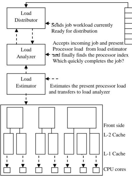
Interconnection structure covers seven virtual processor multi-threaded designed to incorporate parallel behavior. Out of these seven one is tri-core and another is quad core configured, remaining five are of dual core. Fig-1 describes internal structure of workload distribution over core processors along with cache memories and front side disk queue. Several logical component modules exists for final implementation such as load estimator, which periodically measures the load of each processor and a load distributor similarly to load estimator, but whose task is to distribute jobs after analyzing processor present workload. Load distributor is actually the master scheduler cooperatively worked along with load estimator and balances the load.
Jobs Workload
Sends job workload currently Ready for distribution
Accepts incoming job and present Processor load from load estimator
and finally finds the processor index Which quickly completes the job?
Estimates the present processor load and transfers to load analyzer
Front side L-2 Cache
L-1 Cache
CPU cores
[image:2.595.317.545.309.613.2]Fig 1: Multi-Core Interconnection Structure
6.
EFFICIENCY ESTIMATION
Cycle based scheduling requires the calculation of processor’s cycle speed in terms of no. of cycles per second. Fastest processors may pass many no. of cycles in a second as compare to low speed processors [2]. This approach basically computes the no. of cycles elapsed by processor in one second and then measures the amount of time required to compute current job cycles along with the present workload cycles. The load analyzer firstly perform the summation of pending jobs workload cycles from each processor’s ready queue along with the newly arrived job, and then compare it with the
Load Estimator
Load Analyzer
processor cycle speed/sec. Processor having smallest no. of timing requirements for the overall workload will take care of newly arrived job [2]. This will perform the balanced load assignment. The load analyzer finds the processor index as – For each pth processor where p=1 to n
Do
PTotCycleT[p]= (PEloadp + CjobWcycle)*TReqCOneCyclep)
End For
PIndex=Min(PTotCycle) Allocate(Current_Job,PIndex)
7.
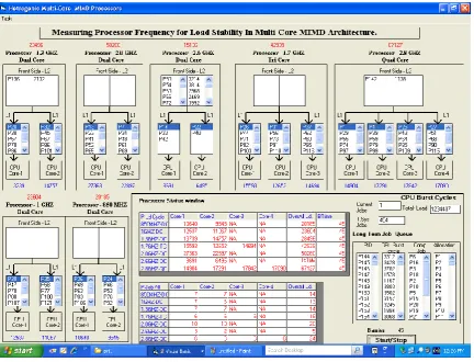
SIMULATED VIEW
Simulated view described below is implemented via visual basic 6.0 programming. The structure represents interconnection among seven multi-core processors along with their workload status details. The underlying logical scenario covers multi-threaded environment along with synchronized communication flow. Each processor having different frequency speed as described in the research. Jobs come under level-2 processor caches described as front end memory bus. Internally the processor manages their cores via level-1 caches buses. The workload is distributed after measurement of processors present workload and cycle speed. Simulator also shows workload of each of the processor core along with overall workload on the basis of which the illustrations have been described. Status logs are also maintained in the database table at different time barriers for analysis. Fig-11 depicts the simulated running view of multi-core processors.
8. MULTI-THREADED ENVIRONMENT
Parallel experimental setup containing simulation structures virtually designed generally covers implementation via multithreading programming, where multiple threads of execution covers each dimension of simulation integral interconnection. In reality, such threads actually executes on a single system but exhibits like they are working as real parallel system covering many interconnected processors cooperatively executes various tasks . Although these threads can be mapped over to actual parallel system, only the logical ability will be distributed among processors. Multi-threading in general requires some sort of synchronization aspects when common shared environment is involved. Experimental setup also covers cluster based parallel execution where no. of machines in a network are incorporated to behave like a parallel system. Such simulated threads can also be mapped to these cluster based architecture with partial modification.9. RESULTS AND DISCUSSIONS
[image:3.595.306.563.71.681.2]Results illustrated below are captured by executing simulation at different distribution samples, where each sample carries different scheduling workload. The research results shows that great amount of efforts is performed at underlying architecture during workload distribution. Load stability and steadiness is controlled at greater extent above to the 85%. As in the illustrations the processor having low frequency rate will processed load according to that as compare to fastest processor with greater frequency speed. Overall load will be balanced. This dynamic approach has the advantage over static scheduling polices. Following are the resultants tables and graphs captured-
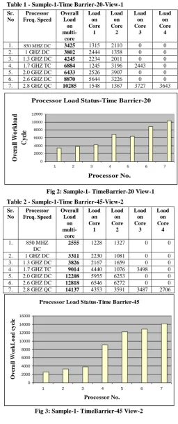
Table 1 - Sample-1-Time Barrier-20-View-1
Sr. No
Processor Freq. Speed
Overall Load
on
multi-core
Load on Core
1
Load on Core
2
Load on Core
3
Load on Core
4
1. 850 MHZ DC 3425 1315 2110 0 0
2. 1 GHZ DC 3802 2444 1358 0 0
3. 1.3 GHZ DC 4245 2234 2011 0 0
4. 1.7 GHZ TC 6884 1245 3196 2443 0
5. 2.0 GHZ DC 6433 2526 3907 0 0
6. 2.6 GHZ DC 8870 5644 3226 0 0
7. 2.8 GHZ QC 10285 1548 1367 3727 3643
[image:3.595.308.564.73.377.2]Fig 2: Sample-1- TimeBarrier-20 View-1
Table 2 - Sample-1-Time Barrier-45-View-2
Sr. No
Processor Freq. Speed
Overall Load
on
multi-core
Load on Core
1
Load on Core
2
Load on Core
3
Load on Core
4
1. 850 MHZ
DC
2555 1228 1327 0 0
2. 1 GHZ DC 3311 2230 1081 0 0
3. 1.3 GHZ DC 3826 2167 1659 0 0
4. 1.7 GHZ TC 9014 4440 1076 3498 0
5. 2.0 GHZ DC 12208 5955 6253 0 0
6. 2.6 GHZ DC 12818 6546 6272 0 0
7. 2.8 GHZ QC 14137 4353 3591 3487 2706
Fig 3: Sample-1- TimeBarrier-45 View-2 Processor Load Status-Time Barrier-20
0 2000 4000 6000 8000 10000 12000
1 2 3 4 5 6 7
Processor No.
O
v
er
a
ll
Wo
rk
lo
a
d
C
y
cl
e
Processor Load Status-Time Barrier-45
0 2000 4000 6000 8000 10000 12000 14000 16000
1 2 3 4 5 6 7
Processor No.
O
v
er
a
ll
Wo
rk
L
o
a
d
c
y
cl
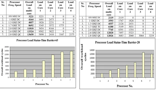
Table 3 - Sample-1-Time Barrier-65-View-3 Table 5 - Sample-2-Time Barrier-20-View-1
Sr. No
Processor Freq. Speed
Overall Load on multi-core Load on Core 1 Load on Core 2 Load on Core 3 Load on Core 4
1. 850 MHZ DC 3221 3221 0 0 0
2. 1 GHZ DC 4164 1691 2473 0 0
3. 1.3 GHZ DC 4057 1826 2231 0 0
4. 1.7 GHZ TC 8692 3345 3572 1775 0
5. 2.0 GHZ DC 11818 3654 8164 0 0
6. 2.6 GHZ DC 13324 9502 3822 0 0
7. 2.8 GHZ QC 13650 5898 2410 3167 2175
[image:4.595.38.560.275.690.2]Fig 4: Sample-1- TimeBarrier-65 View-3
Table 4 - Sample-2-Time Barrier-40-View-2
Sr. No Processor Freq. Speed Overall Load on multi-core Load on Core 1 Load on Core 2 Load on Core 3 Load on Core 4
1. 850 MHZ
DC
3590 1939 1651 0 0
2. 1 GHZ DC 3062 3062 0 0 0
3. 1.3 GHZ DC 4761 1039 3722 0 0
4. 1.7 GHZ TC 6679 1995 2170 2514 0
5. 2.0 GHZ DC 8818 6665 2153 0 0
6. 2.6 GHZ DC 12992 8764 4229 0 0
7. 2.8 GHZ QC 14735 2831 7167 3438 1299
Fig 5: Sample-2- TimeBarrier-40 View-2
Fig 6: Sample-2- TimeBarrier-20 View-1
Table 6 - Sample-2-Time Barrier-80-View-3
Sr. No Processor Freq. Speed Overall Load on multi-core Load on Core 1 Load on Core 2 Load on Core 3 Load on Core 4
1. 850 MHZ
DC
2450 1121 1329 0 0
2. 1 GHZ DC 1511 1511 0 0 0
3. 1.3 GHZ DC 3000 0 3000 0 0
4. 1.7 GHZ TC 4277 1311 1428 1538 0
5. 2.0 GHZ DC 6413 2297 4116 0 0
6. 2.6 GHZ DC 7671 4476 3196 0 0
7. 2.8 GHZ QC 8409 2895 1023 1539 1482
Fig 7: Sample-2- TimeBarrier-80 View-3
Processor Load Status-Time Barrier-65
0 2000 4000 6000 8000 10000 12000 14000 16000
1 2 3 4 5 6 7
Processor No. O v e r a ll w o r k lo a d c y c le s
Processor Load Status-Time Barrier-40
0 2000 4000 6000 8000 10000 12000 14000 16000
1 2 3 4 5 6 7
Processor No.
O v e r a ll Wo r k L o a d C y c leProcessor Load Status-Time Barrier-20
0 2000 4000 6000 8000 10000 12000 14000
1 2 3 4 5 6 7
Processor No.
O v e r a ll w o r k lo a d c y c le sProcessor Load Status-Time Barrier-80
0 2000 4000 6000 8000 10000
1 2 3 4 5 6 7
Processor No. O v e r a ll Wo r k lo a d C y c le s Sr. No Processor Freq. Speed
Overall Load on multi-core Load on Core 1 Load on Core 2 Load on Core 3 Load on Core 4
1. 850 MHZ DC 2119 2119 0 0 0
2. 1 GHZ DC 3593 1767 1826 0 0
3. 1.3 GHZ DC 4557 2126 2431 0 0
4. 1.7 GHZ TC 6180 3149 3031 0 0
5. 2.0 GHZ DC 7745 6391 1354 0 0
6. 2.6 GHZ DC 12820 7497 5323 0 0
Table 7 - Sample-3-Time Barrier-35-View-1 Sr. No Processor Freq. Speed Overall Load on multi-core Load on Core 1 Load on Core 2 Load on Core 3 Load on Core 4
1. 850 MHZ
DC
2931 2931 0 0 0
2. 1 GHZ DC 3484 1152 2332 0 0
3. 1.3 GHZ DC 3523 3523 0 0 0
4. 1.7 GHZ TC 4901 2837 0 2064 0
5. 2.0 GHZ DC 5843 2088 3756 0 0
6. 2.6 GHZ DC 9013 2757 6256 0 0
7. 2.8 GHZ QC 8705 3061 1535 1983 2126
[image:5.595.48.301.75.380.2]Fig 8: Sample-3- TimeBarrier-35 View-1
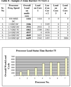
Table 8 - Sample-3-Time Barrier-75-View-2
Sr. No Processor Freq. Speed Overall Load on multi-core Load on Core 1 Loa d on Cor e 2 Load on Core 3 Load on Core 4
1. 850 MHZ
DC
1416 1416 0 0 0
2. 1 GHZ DC 2106 1 2105 0 0
3. 1.3 GHZ DC 2932 2932 0 0 0
4. 1.7 GHZ TC 4462 2100 2362 0 0
5. 2.0 GHZ DC 4937 0 4938 0 0
6. 2.6 GHZ DC 4849 2433 2416 0 0
7. 2.8 GHZ QC 6439 2342 1493 0 2604
Fig 9: Sample-3- TimeBarrier-75 View-2
Table 9 - Sample-3-Time Barrier-95-View-3
Sr. No Processor Freq. Speed Overall Load on multi-core Load on Core 1 Load on Core 2 Load on Core 3 Load on Core 4
1. 850 MHZ
DC
6222 4287 1935 0 0
2. 1 GHZ DC 5628 2280 3348 0 0
3. 1.3 GHZ DC 8230 5345 2885 0 0
4. 1.7 GHZ TC 11108 3588 6488 1032 0
5. 2.0 GHZ DC 13687 5385 8303 0 0
6. 2.6 GHZ DC 17487 10277 7210 0 0
7. 2.8 GHZ QC 19733 4985 7606 1959 5183
Fig 10: Sample-3- TimeBarrier-95 View-3
10.
CONCLUSION AND FUTUREWORK
Conclusion behind this implementation is to balance job distribution in time sharing environment where jobs are encountered frequently and no. of processors are available to handle their processing workload. The results demonstrate that the distribution results are stable upto very high extents nearly 85 to 95 percent. As the graphs shows the each core processors will carrier workload according to their cycle speed and job distribution will be in steadiness state. The processor having lower frequency will no be over burdened or processor with high frequency speed will not be possessed with less workload. So overall distribution will be controlled with consistency. Three different running sampling views are illustrated to show the effects. Future version of this research may consider the further hetro-cores, in which each processor may have different frequency cores. Such architectures are one level above to these because underlying logical aspects of load balancing is increased. Firstly the load is balanced over multi-core MIMD and then each core processor will manage load over their underlying cores by estimating their current load and frequency speed. Simulated implementation will carry great amount of synchronization efforts among processor cores. Load is balanced in two perspectives, either firstly distributes in static fashion and then manages or either during distribution the load mechanisms must be considered along with distribution mechanism, the process is on going, periodically estimates the load and distributes, load analyzers and scheduler work cooperatively to balance the system steady state.
Processor Load Status-Time Barrier-35
0 2000 4000 6000 8000 10000
1 2 3 4 5 6 7
Processor No. O v e r a ll Wo r k L o a d C y c le
Processor Load Status-Time Barrier-75
0 1000 2000 3000 4000 5000 6000 7000
1 2 3 4 5 6 7
Processor No. O v e r a ll Wo r k L o a d C y c le
Processor Load Status-Time Barrier-95
0 5000 10000 15000 20000 25000
1 2 3 4 5 6 7
[image:5.595.50.300.419.722.2]Fig 11: Simulated View
11.
REFERENCES
[1] Srinivasa Rao, P. and Govardhan, 2013 A. Dynamic Load Balancing With Central Monitoring of Distributed Job Processing System. Foundation of Computer Science New York.
[2] Arora, S., Arora, A. 2013. Scheduling simulations: An experimental approach to time-sharing multiprocessor scheduling schemes. Foundation of Computer Science New York
[3] Lokhande, M., Atique, M., 2012. Real-Time Scheduling for Parallel Task Models on Multi-Core Processors-A Critical review”. .
[4] Hager, G. and Wellein, G. 2012 Ingredients for good parallel performance multi-core based systems spring sim, Alexander university Orlando USA
[5] Marowka, A. J. 2011 Back to thin-core massively parallel processors. Bar-llan University, Israel. IEEE computer society.
[6] Varbanescu, A. 2010. On the effective parallel programming on multi-core processors. Universitatea POLITEHNICA Bucuresti Romania
[7] Jurczuk, K. Kretowski, M. 2010 Load balancing in parallel implementation of vascular network modeling.
University of Rennes, France.
[8] Chhabra, A. Singh, G. 2009. Simulated Performance Analysis of Multiprocessor Dynamic Space-Sharing Scheduling policy.
[9] Jaques, M. and Couturier, R. 2005 IEEE, Sylvain Contassot-Vivier, Member, Dynamic Load Balancing and Efficient Load Estimators for Asynchronous Iterative Algorithms
[10]Barker, K. Chernikov, A. 2004 A Load Balancing Framework for Adaptive and Asynchronous Applications. IEEE Transactions on parallel and distributed computing.
[11]Jacques, M. and Contassot, S. 2003. Coupling Dynamic Load Balancing with Asynchronism in Iterative Algorithms on the Computational Grid. IEEE computer society.
[12]Marc, H. Lemair, W.1993. Strategies for load balancing for highly parallel computers IEEE transactions on parallel and distributed systems.
[13]Cybenko, G. 1989. Dynamic load balancing for distributed memory multi-processor Department of Computer Science, Tufts University, Medford, Massachusetts.