R E S E A R C H
Open Access
A quasi-Newton algorithm for large-scale
nonlinear equations
Linghua Huang
**Correspondence: [email protected] School of Information and Statistics, Guangxi University of Finance & Economics, Nanning, Guangxi 530003, P.R. China
Abstract
In this paper, the algorithm for large-scale nonlinear equations is designed by the following steps: (i) a conjugate gradient (CG) algorithm is designed as a sub-algorithm to obtain the initial points of the main algorithm, where the sub-algorithm’s initial point does not have any restrictions; (ii) a quasi-Newton algorithm with the initial points given by sub-algorithm is defined as main algorithm, where a new
nonmonotone line search technique is presented to get the step length
α
k. The givennonmonotone line search technique can avoid computing the Jacobian matrix. The global convergence and the 1 +q-order convergent rate of the main algorithm are established under suitable conditions. Numerical results show that the proposed method is competitive with a similar method for large-scale problems.
Keywords: nonlinear equations; large-scale; conjugate gradient; quasi-Newton method; global convergence
1 Introduction
Consider the following nonlinear equations:
e(x) = , x∈ n. (.)
Heree:n→ nis continuously differentiable andndenotes large-scale dimension. The large-scale nonlinear equations are difficult to solve since the relations of the variables
xare complex and the dimension is larger. Problem (.) can model many real-life prob-lems, such as engineering probprob-lems, dimensions of mechanical linkages, concentrations of chemical species, cross-sectional properties of structural elements, etc. If the Jacobian ∇e(x) ofeis symmetric, then problem (.) is called a system of symmetric nonlinear equa-tions. Letpbe the norm function withp(x) =e(x), where · is the Euclidean norm.
Then (.) is equivalent to the following global optimization models:
minp(x), x∈ n. (.)
In fact, there are many actual problems that can convert to the above problems (.) (see [–] etc.) and have similar models (see [–] etc.). The iterative formula for (.) is
xk+=xk+αkdk,
whereαkis a step length anddkis a search direction. Now let us review some methods for
αkanddk, respectively:
(i) Li and Fukashima [] proposed an approximately monotone technique forαk: p(xk+αkdk) –p(xk)≤–δαkdk–δαkek+kek, (.)
whereek=e(xk),δ> ,δ> are positive constants,αk=rik,r∈(, ),ikis the smallest
nonnegative integerisatisfying (.) andksuch that
∞
k=
k<∞. (.)
(ii) Guet al.[] presented a descent line search technique:
p(xk+αkdk) –p(xk)≤–δαkdk–δαkek. (.)
(iii) Brown and Saad [] gave the following technique to obtainαk:
p(xk+αkdk) –p(xk)≤βαk∇p(xk)Tdk, (.)
whereβ∈(, ) and∇p(xk) =∇e(xk)e(xk).
(iv) Based on this technique, Zhu [] proposed a nonmonotone technique:
p(xk+αkdk) –p(xl(k))≤βαk∇p(xk)Tdk, (.) p(xl(k)) =max≤j≤m(k){p(xk–j)},m() = , andm(k) =min{m(k– ) + ,M},k≥, andMis
a nonnegative integer.
(v) Yuan and Lu [] gave a new technique:
p(xk+αkdk) –p(xk)≤βαke(xk)Tdk, (.)
and some convergence results are obtained.
Next we present some techniques for the calculation ofdk. At present, there exist many
well-known methods fordk, such as the Newton method, the trust region method, and
the quasi-Newton method, etc.
(i) The Newton method has the following form to getdk:
∇e(xk)dk= –e(xk). (.)
This method is regarded as one of the most effective methods. However, its efficiency largely depends on the possibility to efficiently solve (.) at each iteration. Moreover, the exact solution of the system (.) could be too burdensome when the iterative pointxkis far
from the exact solution []. In order to overcome this drawback, inexact quasi-Newton methods are often used.
(ii) The quasi-Newton method is of the form
where Bk is generated by a quasi-Newton update formula, where the BFGS
(Broyden-Fletcher-Goldfarb-Shanno) update formula is one of the well-known quasi-Newton for-mulas with
Bk+=Bk–
BksksTkBk sTkBksk
+ykyk
T
ykTsk
, (.)
wheresk=xk+–xk,yk=ek+–ek, andek+=e(xk+). SetHk to be the inverse ofBk, then
the inverse formula of (.) has the following form:
Hk+=Hk–
ykT(sk–Hkyk)sksTk
(ykTsk)
+(sk–Hkyk)s
T
k +sk(sk–Hkyk)T
(ykTsk)
=
I–skyk
T
ykTsk
Hk
I– yks
T k ykTsk
+ sks
T k ykTsk
. (.)
There exist many quasi-Newton methods (see [, , –]) representing the basic ap-proach underlying most of the Newton-type large-scale algorithms.
The earliest nonmonotone line search framework was developed by Grippo, Lampar-iello, and Lucidi in [] for Newton’s methods. Many subsequent papers have exploited nonmonotone line search techniques of this nature (see [–] etc.), which shows that the nonmonotone technique works well in many cases. Considering these points, Zhu [] proposed the nonmonotone line search (.). From (.), we can see that the Jacobian ma-trix∇e(x) must be computed at every iteration. Computing the Jacobian matrix∇e(x) may be expensive ifnis large and for anynat every iteration. Thus, one might prefer to remove the matrix, leading to a new nonmonotone technique.
Inspired by the above observations, we make a study of inexact quasi-Newton methods with a new nonmonotone technique for solving smooth nonlinear equations. In thekth iteration of our algorithm, the following new nonmonotone technique is used to obtain
αk:
p(xk+αkdk)≤p(xl(k)) +αkσe(xk)Tdk, (.)
whereσ∈(, ) is a constant anddkis a solution of (.). Comparing with (.), the new
equations, where the terminated iteration point of the CG algorithm was used as the ini-tial point of the given algorithm (main algorithm). Then there exist two advantages from this process: one is that we can use the CG’s characteristic to get a better initial point and another is that the good convergent results of the main algorithm can be preserved. The main attributes of this paper are stated as follows:
• A sub-algorithm is designed to get the initial point of the main algorithm. • A new nonmonotone line search technique is presented, moreover, the Jacobian
matrix∇ekmust not be computed at every iteration.
• The given method possesses the sufficient descent property for the normal function
p(x).
• The global convergence and the +q-order convergent rate of the new method are established under suitable conditions.
• Numerical results show that this method is more effective than other similar methods. We organize the paper as follows. In Section , the algorithms are stated. Convergent results are established in Section and numerical results are reported in Section . In the last section, our conclusion is given. Throughout this paper, we use these notations: · is the Euclidean norm,e(xk) andg(xk+) are replaced byekandgk+, respectively.
2 Algorithm
In this section, we will design a sub-algorithm and the main algorithm, respectively. These two algorithms are listed as follows.
Initial point algorithm (sub-algorithm)
Step : Given anyx∈ n,δ,δ∈(, ),k> ,r∈(, ),∈[, ), letk:= .
Step : Ifek ≤, stop. Otherwise letdk= –ekand go to next step.
Step : Choosek+satisfies (.) and letαk= ,r,r,r, . . .until (.) holds.
Step : Letxk+=xk+αkdk.
Step : Ifek+ ≤, stop.
Step : Computedk+= –ek++βkdk, setk=k+ and go to Step .
Remark (i)βkof Step is a scalar and differentβkwill determine different CG methods.
(ii) From Step and [], it is easy to deduce that there existsαksuch that (.). Thus,
this sub-algorithm is well defined.
In the following, we will state the main algorithm. First, assume that the terminated point of sub-algorithm isxsup, then the given algorithm is defined as follows.
Algorithm (Main algorithm) Step: Choose xsup∈ nas the initial point, an initial
symmetric positive definite matrix B∈ n×n,and constants r,σ∈(, ),main<,a posi-tive integer M> ,m(k) = ,let k:= ;
Step : Stop ifek ≤main.Otherwise solve(.)to getdk.
Step : Letαk= ,r,r,r, . . .until(.)holds.
Step : Let the next iterative bexk+=xk+αkdk.
Step : UpdateBkby quasi-Newton update formula and ensure the update matrixBk+
is positive definite.
Remark Step of Algorithm can ensure thatBkis always positive definite. This means
that (.) has a unique solutiondk. By positive definiteness ofBk, it is easy to obtaineTkdk<
. In the following sections, we only concentrate to the convergence of the main algorithm.
3 Convergence analysis Letbe the level set with
=x|e(x)≤e(x). (.) Similar to [, , ], the following assumptions are needed to prove the global conver-gence of Algorithm .
Assumption A (i)eis continuously differentiable on an open convex setcontaining.
(ii) The Jacobian ofeis symmetric, bounded, and positive definite on,i.e., there exist
positive constantsM∗≥m∗> such that
∇e(x)≤M∗ ∀x∈ (.)
and
m∗d≤dT∇e(x)d ∀x∈,d∈ n. (.)
Assumption B Bkis a good approximation to∇ek,i.e.,
(∇ek–Bk)dk≤∗ek, (.)
where∗∈(, ) is a small quantity.
Considering Assumption B and using the von Neumann lemma, we deduce thatBkis
also bounded (see []).
Lemma . Let AssumptionBhold.Then dkis a descent direction of p(x)at xk,i.e.,
∇p(xk)Tdk≤–( –∗)e(xk)
. (.)
Proof By using (.), we get
∇p(xk)Tdk=e(xk)T∇e(xk)dk
=e(xk)T ∇e(xk) –Bk
dk–e(xk)
=e(xk)T ∇e(xk) –Bk
dk–e(xk)Te(xk). (.)
Thus, we have
∇p(xk)Tdk+e(xk)
=e(xk)T ∇e(xk) –Bk
dk
≤e(xk) ∇e(xk) –Bk
It follows from (.) that
∇p(xk)Tdk≤e(xk) ∇e(xk) –Bk
dk–e(xk)
≤–( –∗)e(xk). (.)
The proof is complete.
The following lemma shows that the line search technique (.) is reasonable, then Algorithm is well defined.
Lemma . Let AssumptionsAandBhold.Then Algorithmwill produce an iteration
xk+=xk+αkdkin a finite number of backtracking steps.
Proof From Lemma . in [] we have in a finite number of backtracking steps
p(xk+αkdk)≤p(xk) +αkσe(xk)Tdk,
from which, in view of the definition ofp(xl(k)) =max≤j≤m(k){p(xk–j)} ≥p(xk), we obtain
(.). Thus we conclude the result of this lemma. The proof is complete.
Now we establish the global convergence theorem of Algorithm .
Theorem . Let AssumptionsAandBhold,and{αk,dk,xk+,ek+}be generated by Algo-rithm.Then
lim
k→∞ek= . (.)
Proof By the acceptance rule (.), we have
p(xk+) –p(xl(k))≤σ αkeTkdk< . (.)
Usingm(k+ )≤m(k) + andp(xk+)≤p(xl(k)), we obtain
p(xl(k+))≤max
p(xl(k)),p(xk+)
=p(xl(k)).
This means that the sequence{p(xl(k))}is decreasing for allk. Then{p(xl(k))}is convergent.
Based on Assumptions A and B, similar to Lemma . in [], it is not difficult to deduce that there exist constantsb≥b> such that
bdk≤dkTBkdk= –eTkdk≤bdk. (.)
By (.) and (.), for allk>M, we get
p(xl(k)) =p(xl(k)–+αl(k)–dl(k)–)
≤ max
≤j≤m(l(k)–)
p(xl(k)–j–)
+σ αl(k)–gTl(k)–dl(k)–
≤ max
≤j≤m(l(k)–)
p(xl(k)–j–)
Since{p(xl(k))}is convergent, from the above inequality, we have
lim
k→∞αl(k)–dl(k)–
= .
This implies that either
lim
k→∞infdl(k)–= (.)
or
lim
k→∞infαl(k)–= . (.)
If (.) holds, following [], by induction we can prove that
lim
k→∞dl(k)–j= (.)
and
lim
k→∞p(xl(k)–j) =klim→∞p(xl(k))
for any positive integerj. Ask≥l(k)≥k–MandMis a positive constant, by
xk=xk–M–+αk–M–dk–M–+· · ·+αl(k)–dl(k)–
and (.), it can be derived that
lim
k→∞p(xl(k)) =klim→∞p(xk). (.)
According to (.) and the rule for accepting the stepαkdk,
p(xk+) –p(xl(k))≤αkσeTkdk≤αkσbdk. (.)
This means
lim
k→∞αkdk
= ,
which implies that
lim
k→∞αk= (.)
or
lim
If equation (.) holds, sinceBkis bounded, thenek=Bkdk ≤ Bkdk → holds.
The conclusion of this lemma holds. If (.) holds. Then acceptance rule (.) means that, for all large enoughk,αk=αk
r such that
p xk+αkdk
–p(xk)≥pxk+αkdk
–p(xl(k)) >σ αkeTkdk. (.)
Since
p xk+αkdk
–p(xk) =αk∇p(xk)Tdk+o αkdk
. (.)
Using (.) and (.) in [], we have
∇p(xk)Tdk=eTk∇e(xk)dk≤δ∗eTkdk,
whereδ∗> is a constant andσ<δ∗. So we get
δ∗–σαkeTkdk+o αkdk
≥. (.)
Note thatδ∗–σ> andeT
kdk< , we have from dividing (.) byαkdk
lim
k→∞
eTkdk
dk
= . (.)
By (.), we have
lim
k→∞dk= . (.)
Consider ek = Bkdk ≤ Bkdk and the bounded Bk again, we complete the
proof.
Lemma .(see Lemma . in []) Let e be continuously differentiable,and∇e(x)be
nonsingular at x∗which satisfies e(x∗) = .Let
a≡∇e x∗+ c, c
,c=∇e x∗–. (.)
Ifxk–x∗sufficiently small,then the inequality
axk–x
∗≤e(x
k)≤axk–x∗ (.)
holds.
Theorem . Let the assumptions in Lemma.hold.Assume that there exists a
suffi-ciently smallε> such thatBk–∇e(xk) ≤εfor each k.Then the sequence{xk} con-verges to x∗superlinearly forαk= .Moreover,if e is q-order smooth at x∗ and there is a neighborhood U of x∗satisfying for any xk∈U,
Bk–∇e x∗ xk–x∗≤ηxk–x∗
+q
, (.)
Proof Sincegis continuously differentiable and∇e(x) is nonsingular atx∗, there exists a constantγ > and a neighborhoodUofx∗satisfying
max∇e(y),∇e(y)–≤γ,
where∇e(y) is nonsingular for anyy∈U. Consider the following equality whenαk= : Bk xk+–x∗
+∇e(xk)xk–x∗
–Bk xk–x∗
+e(xk) –e x∗
–∇e(xk) xk–x∗
=e(xk) +Bkdk= , (.)
the second term and the third term areo(xk–x∗). By the von Neumann lemma, and
considering that∇e(xk) is nonsingular,Bkis also nonsingular. For anyy∈U and∇e(y)
being nonsingular andmax{∇e(y),∇e(y)–} ≤γ, then we obtain from Lemma .
xk+–x∗=o xk–x∗=o e(xk), ask→ ∞,
this means that the sequence{xk}converges tox∗superlinearly forαk= .
Ifeisq-order smooth atx∗, then we get
e(xk) –e x∗
–∇e(xk)xk–x∗
=O xk–x∗ q+
.
Consider the second term of (.) as xk→x∗, and use (.), we can deduce that the
second term of (.) is alsoO(xk–x∗q+). Therefore, we have
xk+–x∗=O xk–x∗
q+
, asxk→x∗.
The proof is complete.
4 Numerical results
In this section, we report results of some numerical experiments with the proposed method. The test functions have the following form:
e(x) = f(x),f(x), . . . ,fn(x)
T
,
where these functions have the associated initial guessx. These functions are stated as follows.
Function Exponential function
f(x) =ex– ,
fi(x) = i
e
xi+x
i––
, i= , , . . . ,n.
Function Trigonometric function
fi(x) =
n+i( –cosxi) –sinxi– n
j=
cosxj
(sinxi–cosxi), i= , , , . . . ,n.
Initial guess:x= (n,n, . . . ,n)T.
Function Logarithmic function
fi(x) =ln(xi+ ) – xi
n, i= , , , . . . ,n.
Initial guess:x= (, , . . . , )T.
Function Broyden tridiagonal function [[], pp. -]
f(x) = ( – .x)x– x+ ,
fi(x) = ( – .xi)xi–xi–+ xi++ ,
i= , , . . . ,n– ,
fn(x) = ( – .xn)xn–xn–+ .
Initial guess:x= (–, –, . . . , –)T.
Function Trigexp function [[], p. ]
f(x) = x+ x– +sin(x–x)sin(x+x),
fi(x) = –xi–exi––xi+xi + xi
+ xi+
+sin(xi–xi+)sin(xi+xi+) – , i= , , . . . ,n– ,
fn(x) = –xn–exn––xn+ xn– .
Initial guess:x= (, , . . . , )T.
Function Strictly convex function [[], p. ].e(x) is the gradient ofh(x) =ni=(exi– xi).
fi(x) =exi– , i= , , , . . . ,n.
Initial guess:x= (n,n, . . . , )T.
Function Strictly convex function [[], p. ]
e(x) is the gradient ofh(x) =ni= i
(e
xi–x
i).
fi(x) = i
e
xi– , i= , , , . . . ,n.
Function Variable dimensioned function
fi(x) =xi– , i= , , , . . . ,n– ,
fn–(x) = n–
j=
j(xj– ),
fn(x) =
n–
j=
j(xj– )
.
Initial guess:x= ( –n, –n, . . . , )T.
Function Discrete boundary value problem [].
f(x) = x+ .h(x+h)–x,
fi(x) = xi+ .h(xi+hi)–xi–+xi+,
i= , , . . . ,n–
fn(x) = xn+ .h(xn+hn)–xn–,
h=
n+ .
Initial guess:x= (h(h– ),h(h– ), . . . ,h(nh– )).
Function The discretized two-point boundary value problem similar to the problem
in []
e(x) =Ax+
(n+ )F(x) = ,
whenAis then×ntridiagonal matrix given by
A= ⎡ ⎢ ⎢ ⎢ ⎢ ⎢ ⎢ ⎢ ⎢ ⎢ ⎢ ⎣
– – –
– – . .. ... ...
. .. ... – –
⎤ ⎥ ⎥ ⎥ ⎥ ⎥ ⎥ ⎥ ⎥ ⎥ ⎥ ⎦ ,
and F(x) = (F(x),F(x), . . . ,Fn(x))T with Fi(x) =sinxi – ,i= , , . . . ,n, andx= (, ,
, , . . .).
with initial pointsx(called the normal method). Aslam Nooret al.[] presented a vari-ational iteration technique for nonlinear equations, where the so-called VIM method has the better numerical performance. The VIM method has the following iteration form:
xk+=xk–
∇e– diag(βe,βe, . . . ,βnen)
–
(xk)e(xk),
whereβi∈(, ) fori= , , . . . ,n. In their paper, only low dimension problems (two
vari-ables) are tested. In this experiment, we also give the numerical results of this method for large-scale nonlinear equations to compare with our proposed algorithm.
The parameters were chosen asr= .,σ= .,M= ,= –, and
main= –. In
order to ensure the positive definiteness ofBk, in Step of the main algorithm: ifyTksk>
, updateBk by (.), otherwise letBk+=Bk. This program will also be stopped if the
iteration number of main algorithm is larger than . Since the line search cannot always ensure these descent conditionsdkTek< anddkT∇e(xk)ek< , an uphill search direction
may occur in numerical experiments. In this case, the line search rule maybe fails. In order to avoid this case, the stepsizeαkwill be accepted if the searching time is larger than six
in the inner circle for the test problems.
In the sub-algorithm, the CG formula is used by the following Polak-Ribière-Polyak (PRP) method [, ]
dk=
⎧ ⎨ ⎩
–ek+
eTk(ek–ek–)
ek– dk– ifk≥,
–ek ifk= .
(.)
For the line search technique, (.) is used and the largest search number of times is ten, whereδ=δ= –, andk=NI (NIis the iteration number). The sub-algorithm will
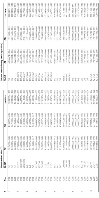
also stopped if the iteration number is larger than . The iteration number, the function evaluations, and the CPU time of the sub-algorithm are added to the main algorithm for new method with CG. The meaning of the items of the columns of Table is:
Dim: the dimension.
NI: the number of iterations.
NG: the number of function evaluations. cpu time: the cpu time in seconds.
GF: the final norm function evaluationsp(x) when the program is stopped. GD: the final norm evaluations of search directiondk.
fails: fails to find the final values ofp(x) when the program is stopped.
From Tables -, it is easy to see that the number of iterations and the number of function evaluations of the new method with CG are less than those of the normal method for these test problems. Moreover, the cpu time and the final function norm evaluations of the new method with CG are more competitive than those of the normal method. For the VIM method, the results of Problems - are very interesting, but it fails for Problems -. Moreover, it is not difficult to find that more CUP time is needed for this method. The main reason maybe lies in the computation of the Jacobian matrix at every iteration.
The tool of Dolan and Moré [] is used to analyze the efficiency of these three algo-rithms.
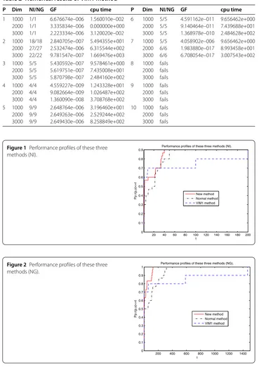
Table 2 Numerical results of VIM1 method
P Dim NI/NG GF cpu time P Dim NI/NG GF cpu time
1 1000 1/1 6.676674e–006 1.560010e–002 6 1000 5/5 4.591162e–011 9.656462e+000 2000 1/1 3.335834e–006 0.000000e+000 2000 5/5 9.140464e–011 7.439688e+001 3000 1/1 2.223334e–006 3.120020e–002 3000 5/5 1.368978e–010 2.484628e+002 2 1000 18/18 2.840705e–007 5.494355e+001 7 1000 5/5 4.058902e–006 9.656462e+000 2000 27/27 2.532474e–006 6.315544e+002 2000 6/6 1.983880e–017 8.993458e+001 3000 22/22 9.781547e–007 1.669476e+003 3000 6/6 6.708054e–017 3.007543e+002 3 1000 5/5 5.430592e–007 9.578461e+000 8 1000 fails
2000 5/5 5.619751e–007 7.435008e+001 2000 fails 3000 5/5 5.870798e–007 2.484160e+002 3000 fails 4 1000 4/4 4.559227e–009 1.243328e+001 9 1000 fails 2000 4/4 9.082664e–009 1.026487e+002 2000 fails 3000 4/4 1.360090e–008 3.708768e+002 3000 fails 5 1000 9/9 2.648764e–006 3.196460e+001 10 1000 fails 2000 9/9 2.649263e–006 2.529244e+002 2000 fails 3000 9/9 2.649430e–006 8.258849e+002 3000 fails
Figure 1Performance profiles of these three methods (NI).
Figure 2Performance profiles of these three methods (NG).
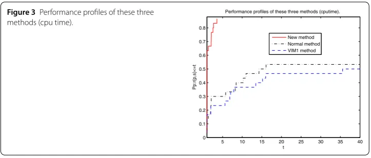
performs best among these three methods. To this end, we think that the enhancement of this proposed method is noticeable.
5 Conclusion
Figure 3Performance profiles of these three methods (cpu time).
Jacobian matrix, a nonmonotone line search technique was used in the algorithms. The convergence results are established and numerical results are reported.
According to the numerical performance, it is clear that the CG technique is very ef-fective for large-scale nonlinear equations. This observation inspires us to design the CG methods to directly solve nonlinear equations in the future.
Competing interests
The author declares to have no competing interests.
Acknowledgements
Only the author contributed in writing this paper. The author thanks the referees and the Editor for their valuable comments, which greatly improved the paper.
Received: 24 November 2016 Accepted: 18 January 2017 References
1. Chen, B, Shu, H, Coatrieux, G, Chen, G, Sun, X, Coatrieux, J: Color image analysis by quaternion-type moments. J. Math. Imaging Vis.51, 124-144 (2015)
2. Fu, Z, Ren, K, Shu, J, Sun, X, Huang, F: Enabling personalized search over encrypted outsourced data with efficiency improvement. IEEE Trans. Parallel Distrib. Syst. (2015). doi:10.1109/TPDS.2015.2506573
3. Gu, B, Sheng, VS: A robust regularization path algorithm forν-support vector classification. IEEE Trans. Neural Netw. Learn. Syst. (2016). doi:10.1109/TNNLS.2016.2527796
4. Gu, B, Sheng, VS, Tay, KY, Romano, W, Li, S: Incremental support vector learning for ordinal regression. IEEE Trans. Neural Netw. Learn. Syst.26, 1403-1416 (2015)
5. Guo, P, Wang, J, Li, B, Lee, S: A variable threshold-value authentication architecture for wireless mesh networks. J. Internet Technol.15, 929-936 (2014)
6. Li, J, Li, X, Yang, B, Sun, X: Segmentation-based image copy-move forgery detection scheme. IEEE Trans. Inf. Forensics Secur.10, 507-518 (2015)
7. Pan, Z, Zhang, Y, Kwong, S: Efficient motion and disparity estimation optimization for low complexity multiview video coding. IEEE Trans. Broadcast.61, 166-176 (2015)
8. Shen, J, Tan, H, Wang, J, Wang, J, Lee, S: A novel routing protocol providing good transmission reliability in underwater sensor networks. J. Internet Technol.16, 171-178 (2015)
9. Xia, Z, Wang, X, Sun, X, Wang, Q: A secure and dynamic multi-keyword ranked search scheme over encrypted cloud data. IEEE Trans. Parallel Distrib. Syst.27, 340-352 (2015)
10. Fu, Z, Wu, X, Guan, C, Sun, X, Ren, K: Towards efficient multi-keyword fuzzy search over encrypted outsourced data with accuracy improvement. IEEE Trans. Inf. Forensics Secur. (2016). doi:10.1109/TIFS.2016.2596138
11. Gu, B, Sun, X, Sheng, VS: Structural minimax probability machine. IEEE Trans. Neural Netw. Learn. Syst. (2016). doi:10.1109/TNNLS.2016.2544779
12. Ma, T, Zhou, J, Tang, M, Tian, Y, Al-Dhelaan, A, Al-Rodhaan, M, Lee, S: Social network and tag sources based augmenting collaborative recommender system. IEICE Trans. Inf. Syst.98, 902-910 (2015)
13. Ren, Y, Shen, J, Wang, JN, Han, J, Lee, S: Mutual verifiable provable data auditing in public cloud storage. J. Internet Technol.16, 317-323 (2015)
14. Yuan, G: Modified nonlinear conjugate gradient methods with sufficient descent property for large-scale optimization problems. Optim. Lett.3, 11-21 (2009)
15. Yuan, G, Duan, X, Liu, W, Wang, X, et al.: Two new PRP conjugate gradient algorithms for minimization optimization models. PLoS ONE10, e0140071 (2015)
16. Yuan, G, Lu, X: A modified PRP conjugate gradient method. Ann. Oper. Res.166, 73-90 (2009)
18. Yuan, G, Wei, Z: New line search methods for unconstrained optimization. J. Korean Stat. Soc.38, 29-39 (2009) 19. Yuan, G, Wei, Z: The superlinear convergence analysis of a nonmonotone BFGS algorithm on convex objective
functions. Acta Math. Sin. Engl. Ser.24(1), 35-42 (2008)
20. Yuan, G, Wei, Z: Convergence analysis of a modified BFGS method on convex minimizations. Comput. Optim. Appl.
47, 237-255 (2010)
21. Yuan, G, Wei, Z: A trust region algorithm with conjugate gradient technique for optimization problems. Numer. Funct. Anal. Optim.32, 212-232 (2011)
22. Yuan, G, Wei, Z: The Barzilai and Borwein gradient method with nonmonotone line search for nonsmooth convex optimization problems. Math. Model. Anal.17, 203-216 (2012)
23. Yuan, G, Wei, Z, Wang, Z: Gradient trust region algorithm with limited memory BFGS update for nonsmooth convex minimization. Comput. Optim. Appl.54, 45-64 (2013)
24. Yuan, G, Wei, Z, Wu, Y: Modified limited memory BFGS method with nonmonotone line search for unconstrained optimization. J. Korean Math. Soc.47, 767-788 (2010)
25. Yuan, G, Wei, Z, Zhao, Q: A modified Polak-Ribière-Polyak conjugate gradient algorithm for large-scale optimization problems. IIE Trans.46, 397-413 (2014)
26. Yuan, G, Zhang, M: A modified Hestenes-Stiefel conjugate gradient algorithm for large-scale optimization. Numer. Funct. Anal. Optim.34, 914-937 (2013)
27. Zhang, Y, Sun, X, Baowei, W: Efficient algorithm for K-barrier coverage based on integer linear programming. China Communications13, 16-23 (2016)
28. Li, D, Fukushima, M: A global and superlinear convergent Gauss-Newton-based BFGS method for symmetric nonlinear equations. SIAM J. Numer. Anal.37, 152-172 (1999)
29. Gu, G, Li, D, Qi, L, Zhou, S: Descent directions of quasi-Newton methods for symmetric nonlinear equations. SIAM J. Numer. Anal.40, 1763-1774 (2002)
30. Brown, PN, Saad, Y: Convergence theory of nonlinear Newton-Krylov algorithms. SIAM J. Optim.4, 297-330 (1994) 31. Zhu, D: Nonmonotone backtracking inexact quasi-Newton algorithms for solving smooth nonlinear equations. Appl.
Math. Comput.161, 875-895 (2005)
32. Yuan, G, Lu, X: A new backtracking inexact BFGS method for symmetric nonlinear equations. Comput. Math. Appl.55, 116-129 (2008)
33. Nash, SG: A surey of truncated-Newton matrices. J. Comput. Appl. Math.124, 45-59 (2000)
34. Dembao, RS, Eisenstat, SC, Steinaug, T: Inexact Newton methods. SIAM J. Numer. Anal.19, 400-408 (1982) 35. Griewank, A: The ’global’ convergence of Broyden-like methods with a suitable line search. J. Aust. Math. Soc. Ser. B,
Appl. Math28, 75-92 (1986)
36. Ypma, T: Local convergence of inexact Newton methods. SIAM J. Numer. Anal.21, 583-590 (1984) 37. Yuan, G, Wei, Z, Lu, X: A BFGS trust-region method for nonlinear equations. Computing92, 317-333 (2011) 38. Yuan, G, Wei, Z, Lu, S: Limited memory BFGS method with backtracking for symmetric nonlinear equations. Math.
Comput. Model.54, 367-377 (2011)
39. Yuan, G, Yao, S: A BFGS algorithm for solving symmetric nonlinear equations. Optimization62, 82-95 (2013) 40. Grippo, L, Lampariello, F, Lucidi, S: A nonmonotone line search technique for Newton’s method. SIAM J. Numer. Anal.
23, 707-716 (1986)
41. Birgin, EG, Martinez, JM, Raydan, M: Nonmonotone spectral projected gradient methods on convex sets. SIAM J. Optim.10, 1196-1211 (2000)
42. Han, J, Liu, G: Global convergence analysis of a new nonmonotone BFGS algorithm on convex objective functions. Comput. Optim. Appl.7, 277-289 (1997)
43. Liu, G, Peng, J: The convergence properties of a nonmonotonic algorithm. J. Comput. Math.1, 65-71 (1992) 44. Zhou, J, Tits, A: Nonmonotone line search for minimax problem. J. Optim. Theory Appl.76, 455-476 (1993) 45. Yuan, G: A new method with descent property for symmetric nonlinear equations. Numer. Funct. Anal. Optim.31,
974-987 (2010)
46. Yuan, G, Meng, Z, Li, Y: A modified Hestenes and Stiefel conjugate gradient algorithm for large-scale nonsmooth minimizations and nonlinear equations. J. Optim. Theory Appl.168, 129-152 (2016)
47. Yuan, G, Lu, S, Wei, Z: A new trust-region method with line search for solving symmetric nonlinear equations. Int. J. Comput. Math.88, 2109-2123 (2011)
48. Yuan, G, Wei, Z, Li, G: A modified Polak-Ribière-Polyak conjugate gradient algorithm for nonsmooth convex programs. J. Comput. Appl. Math.255, 86-96 (2014)
49. Yuan, G, Zhang, M: A three-terms Polak-Ribière-Polyak conjugate gradient algorithm for large-scale nonlinear equations. J. Comput. Appl. Math.286, 186-195 (2015)
50. Yuan, G, Lu, X, Wei, Z: BFGS trust-region method for symmetric nonlinear equations. J. Comput. Appl. Math.230, 44-58 (2009)
51. Gomez-Ruggiero, M, Martinez, J, Moretti, A: Comparing algorithms for solving sparse nonlinear systems of equations. SIAM J. Sci. Comput.23, 459-483 (1992)
52. Raydan, M: The Barzilai and Borwein gradient method for the large scale unconstrained minimization problem. SIAM J. Optim.7, 26-33 (1997)
53. Moré, J, Garbow, B, Hillström, K: Testing unconstrained optimization software. ACM Trans. Math. Softw.7, 17-41 (1981) 54. Aslam Noor, M, Waseem, M, Inayat Noor, K, Al-Said, E: Variational iteration technique for solving a system of nonlinear
equations. Optim. Lett.7, 991-1007 (2013)
55. Polak, E, Ribière, G: Note sur la convergence de directions conjugees. Rev. Franaise Informat. Recherche Opérationnelle3, 35-43 (1969)
56. Polyak, E: The conjugate gradient method in extremal problems. USSR Comput. Math. Math. Phys.9, 94-112 (1969) 57. Dolan, ED, Moré, JJ: Benchmarking optimization software with performance profiles. Math. Program.91, 201-213