Solving a class of generalized fractional programming problems using the feasibility of linear programs

R E S E A R C H

Open Access

Solving a class of generalized fractional

programming problems using the feasibility

of linear programs

Peiping Shen

_{, Tongli Zhang and Chunfeng Wang}

*_{Correspondence: [email protected]} College of Mathematics and Information Science, Henan Normal University, Xinxiang, 453007, P.R. China

Abstract

This article presents a new approximation algorithm for globally solving a class of generalized fractional programming problems (P) whose objective functions are defined as an appropriate composition of ratios of affine functions. To solve this problem, the algorithm solves an equivalent optimization problem (Q) via an exploration of a suitably defined nonuniform grid. The main work of the algorithm involves checking the feasibility of linear programs associated with the interesting grid points. It is proved that the proposed algorithm is a fully polynomial time approximation scheme as the ratio terms are fixed in the objective function to problem (P), based on the computational complexity result. In contrast to existing results in literature, the algorithm does not require the assumptions on

quasi-concavity or low-rank of the objective function to problem (P). Numerical results are given to illustrate the feasibility and effectiveness of the proposed algorithm.

MSC: 90C30; 90C33; 90C15

Keywords: generalized fractional programming; global optimization; approximation algorithm; computational complexity

1 Introduction

In a variety of applications, we encounter a class of nonconvex optimization problems as follows:

(P) : ⎧ ⎨ ⎩

minf(x) =G(cx+c

d_x+d,

c_x+c

d_x+d, . . . ,

cpx+cp

dpx+dp)

s.t. x∈={x∈Rn:Ax≤b,x≥},

where ci,di∈Rn, ci,di ∈R, A∈Rm×n, b ∈Rm, cix+ci> , di x+di >  over a nonempty, compact setfor eachi= , . . . ,p, andG:Rp+→R+is a continuous function.

Problem (P) is worth studying because some important special optimization problems that have been studied in literature fall into the category of (P), such as multiplicative programs, sum-of-ratios optimization, fractional polynomial optimization, namely:

(a) Multiplicative programs (MP): In this case, the objective functionG, with the form G(y, . . . ,yp) =

p

i=yiwithyi= c_ix+ci

dix+di, is quasi-concave, and its minimum is

attained at some extreme point of the polytope []. Multiplicative objective functions arise in a variety of practical applications, such as economic analysis [], robust optimization [], VLSI chip design [], combination optimization [], etc. (b) Sum-of-ratios (SOR) optimization: SOR functions have the form

G(y, . . . ,yp) = p

i=yiwithyi= c_ix+ci

d_ix+di. Matsui [] points out that it is NP-hard to

minimize SOR functions over a polytope. For many applications of this form, we can see the survey paper by Schaible and Shi [] and the references therein. Specially, a kind of SOR optimization problems with the form

G(y, . . . ,yp) = p

i=|yi|q, whereq≥andyi= c_ix+ci

d_ix+di, are considered by Kuno and

Masaki [] as well, and they often occur in a computer version.

(c) Fractional polynomial optimization: Polynomial functions with positive coefficients have the formG(y, . . . ,yp) =

m

j=cj p

i=y γij

i , whereyi= c_ix+ci

d_ix+di,cj≥andγijis a

positive integer. Problems of this form have many applications [], including production planning, engineering design, etc. In addition, from research point of view, these problems pose significant theoretical and computational challenges because they possess multiple local optima that are not globally optima.

During the past years, many solution methods have been developed for globally solving special cases of problem (P). These methods can be classified into outer-approximation [], branch-and-bound [–], mixed branch-and-bound and outer-approximation [], cutting plane [], parameter-based [], vertex enumeration [], heuristic methods [], etc. However, most of these methods lack theoretical analysis of the running time of the algorithms, or performance guarantee of the solutions obtained. To our knowledge, lit-tle work has been done about the solution ofε-approximation problems of (P) without the quasi-concavity and low-rank assumptions; although Locatelli [] has developed an approximation algorithm for a general class of global optimization problems. Next, we immediately introduce the definition of theε-approximation problem related to global optimization as follows.

Definition  Given ε> , letting f∗ =minx∈f(x), a point x¯ ∈ is said to be an ε-approximation solution forminx∈f(x) if

f(x¯)≤f∗+ε|f∗|.

This article focuses on presenting a fully polynomial time approximation scheme (FP-TAS) for solving problem (P). An FPTAS for a minimization problem is an approximation algorithm, that is, for any givenε> , it can find anε-approximation solution for the prob-lem, and its running time is polynomial in the input size of the problem and /ε. As shown by Mittal and Schulz [], the optimum value of problem (P) cannot be approximated to within any factor unlessNP=P. Therefore, in order to obtain an FPTAS for solving prob-lem (P), some extra assumptions of the functionGwill be required (see Section ) in this article.

Ravi [] exploited the fact that the minimum of a quasi-concave function is attained at an extreme point of the polytope and proposed an FPTAS for minimizing a class of low-rank quasi-concave functions over a convex set. Mittal and Schulz [] developed an FPTAS for optimizing a class of low-rank nonconvex functions without quasi-concavity over a polytope. In addition, Depetrini et al. [] and Goyal et al. [] respectively gave an FPTAS for a class of optimization problems where the objective functions are products of two linear functions. Shen and Wang [] presented a linear decomposition approximation algorithm for a class of nonconvex programming problems by dividing the input space into polynomially many grids. Nevertheless, these solution methods [, , –] cannot be directly applied to the case (i.e., problem (P)) considered in this paper, where the objective function is a composition of some ratios of affine functions without quasi-concavity or low-rank.

The aim of this article is to present a solution approach for a class of fractional pro-gramming problems (P). By introducing some variables, the original problem (P) is first converted to ap-dimensional equivalent problem (Q). Through the establishment of a nonuniform grid, on the basis of problem (Q), the solving process of the original prob-lem (P) is then transformed into checking the feasibility of a series of linear programming problems. Thus, a new approximation algorithm is presented for globally solving problem (P) based on the exploration technique of a nonuniform grid over a box. The algorithm does not require quasi-concavity or low-rank of the functionGto problem (P), and it is proved that this is an FPTAS as the termpis fixed inG. We emphasize here that the explo-ration technique used in this article is different from the ones given in [, ]. The reason is that we utilize a different strategy from that given in [, ] to update the incumbent best value of the objective functiong(t) to problem (Q), and that requires fewer interesting grid points restored and considered in our algorithm, compared with Refs. [, ]. Also, we notice that the main computational cost of the proposed algorithm is checking the fea-sibility of linear problems at the interesting grid points. This means that it requires less computational cost and so is more easily implementable. Finally, problem (P) generalizes the one investigated in [], and the proposed algorithm can be directly applied to solve the problem in [] by replacing the convex feasibility with the linear one. Numerical re-sults show that the proposed algorithm requires much less computational time to obtain an approximation optimized solution of problem (P) with the same approximation error than the approaches (given by [, ]) do.

The paper is structured as follows. In Section , we discuss the reformulation of problem (P) as ap-dimensional one. Section  presents an approximation algorithm to obtain an ε-approximation solution for problem (P) which is FPTAS by its computational complexity. Some numerical results are reported in Section . Finally, the conclusions are presented in Section .

2 Parametric reformulation of the problem

For solving problem (P), throughout this paper, we assume thatGsatisfies: • G(y)≤G(y)for ally,y∈Rp+withyi≤yi,i= , . . . ,p, and

• δk_{G(y)≤G(δy)for ally∈R}p

+,∀δ∈(, ), and some constantk.

problem (P) under the above assumptions. For this purpose, let us introducepvariables

yi,i= , . . . ,p, thus, problem (P) can be equivalent to the form:

(P) : ⎧ ⎪ ⎪ ⎪ ⎨ ⎪ ⎪ ⎪ ⎩

minG(y) s.t. cix+ci

d_ix+di≤yi, i= , . . . ,p,

x∈.

Theorem  x∗is a global optimal solution for problem(P)if and only if(x∗,y∗)is a global

optimal solution for problem(P)with y∗_i = cix∗+ci

d_ix∗+di for each i= , . . . ,p.The minimal

ob-jective function values of problems(P)and(P)are equal,i.e.,f(x∗) =G(y∗).

Proof Let (x∗,y∗) be a global optimal solution for problem (P). We suppose thatx∗is not a global optimal solution for problem (P), then there existsx¯∈such that

f(x¯) <fx∗ . (.)

Lety¯i= c_ix+c¯ i

d_ix+d¯ i,i= , . . . ,p. Then (x¯,¯y) is a feasible solution of problem (P). We can have,

from (.), that

G(y¯) =f(x¯) <fx∗ . (.)

On the other hand, since (x∗,y∗) is a feasible solution of problem (P), this implies that c_ix∗+ci

d_ix∗+di≤y ∗

i,i= , . . . ,p. Therefore, from the assumptions ofG, it holds that

fx∗ =G

c_x∗+c

d_x∗+d , c

x∗+c

d_x∗+d , . . . , c

px∗+cp

d_px∗+dp

≤Gy∗ . (.)

Combining (.) with (.), we can obtainG(y¯) <G(y∗). Since (x¯,y¯) is a feasible solution of problem (P), this contradicts the optimality of (x∗,y∗) for problem (P). Therefore, the supposition thatx∗is not a global optimal solution for problem (P) must be false.

Next, we will show the converse case. Letx∗ be a global optimal solution of problem (P), and lety∗_i = cix∗+ci

d_ix∗+di,i= , . . . ,p. Then (x

∗_,y∗_{) is a feasible solution of problem (P).}

Suppose that there exists some feasible solution (x¯,y¯) for problem (P) such that

G(y¯) <Gy∗ =fx∗ . (.)

Then, from cix+c¯ i

d_ix+d¯ i≤ ¯yi,i= , . . . ,p, it follows that

f(x¯) =G

cx¯+c

d_x¯+d , c

x¯+c

d_x¯+d , . . . ,c

px¯+cp

d_px¯+dp

≤G(y¯). (.)

Based on the above theorem, for solving problem (P), we may solve problem (P) instead. Additionally, it is known that each single ratio cix+ci

d_ix+di is both concave and

quasi-convex, and its minimum and maximum must be attained respectively at some vertex of (see, e.g., []). To this end, let us denote

li=min x∈

c_ix+ci

d_ix+di

, ui=max x∈

c_ix+ci

d_ix+di

, i= , . . . ,p. (.)

And let

H=y∈Rp:li≤yi≤ui,i= , . . . ,p

.

Now, let us define ap-dimensional set for eacht∈Has follows:

S(t) =x∈:c_ix+ci≤ti

d_i x+di ,i= , . . . ,p

,

and the corresponding functiong(t) is given by

g(t) = ⎧ ⎨ ⎩

G(t), ifS(t)=∅, +∞, otherwise.

Clearly, we can know whetherS(t) is a null set or not by checking the feasibility of a linear program for givent∈H, which can be solved in polynomial time. Based on the above result, it turns out that problem (P) is equivalent to the followingp-dimensional problem:

(Q) : min t∈Hg(t).

According to the definition ofg(t), we have the following conclusion.

Theorem  Givenε> ,letδ= (_+ε )/k,for each¯t∈H,it holds that

g(¯t)≤( +ε)g(t), ∀t∈[δ¯t,t¯].

Proof From the definition ofS(t) andδ= (_+ε )/k_{∈(, ), we haveS(δ}¯_t)⊆S(t¯_{) for each}

¯

t∈H. WhenS(δt¯)=∅, it implies thatS(t)=∅for eacht∈[δt¯,¯t]. This means thatg(t) =G(t) for eacht∈[δt¯,¯t]. With the assumptions ofG(t), it holds that

( +ε)g(t) = ( +ε)G(t)≥( +ε)G(δt¯)≥( +ε)δkG(¯t) =G(¯t) =g(t¯), ∀t∈[δ¯t,t¯].

WhenS(δ¯t) =∅andS(¯t)=∅, similarly, we have that

( +ε)g(t)≥( +ε)G(t)≥( +ε)G(δ¯t)≥( +ε)δk_G(¯_{t) =G(}¯_{t) =g(t}¯_{), ∀t∈[δ}¯_t,¯_t].

3 The approximation algorithm

3.1 The algorithm and its convergence

In this subsection, by using Theorem  above, we present an approximation algorithm for solving problem (P), and prove that the algorithm can find anε-approximation solution for problem (P).

The proposed algorithm adopts an exploration technique of a suitably defined nonuni-form grid overH. In the algorithm, letT be the set of all restored interesting grid points which will be further analyzed.W is a set of the grid points already discarded, andX is a set of the remaining grid points at each iteration. Moreover,U represents the best value of the functiong(t) obtained so far, and denotet∗ such thatU=g(t∗). The algo-rithm starts witht∗= (u, . . . ,up) andU=g(t∗). In each iteration, we select a point¯t∈T

and calculatea¯=min{a∈N:S(δa¯_{t) =∅}, whereNrepresents the set of the natural} num-bers. Ifa¯= , we newly select a point¯tfromT. Otherwise, we haveS(δa–¯ ¯_{t)=∅, and so}

S(t)=∅for eacht∈[δa–¯ ¯_t,¯_{t]. This implies thatg(t) =G(t) for eacht∈[δ}a–¯ _t¯_,¯_{t]. By using} the nondecreasingG, it holds thatg(δa–¯ _t¯_{) =min}

t∈[δa¯–_¯t,t]¯ g(t). In addition, for anyt∈ {t:

δa¯_t¯

i<ti≤ ¯ti,i= , . . . ,p}(δa¯t¯,¯t], there exists an integer vectorτ = (τ, . . . ,τp) such that

ti∈(δτi+¯ti,δτi¯ti] satisfyingτi∈ {, , . . . ,a¯– }for eachi, thus, we have ( +ε)g(t)≥g(δτ¯t) for anyt∈(δτ+¯_t,δτ¯_{t] from Theorem . We see that all pointsδ}τ¯_{t= (δ}τ_t¯_{, . . . ,δ}τp¯_t

p) with τi∈ {, , . . . ,a¯– }belong to [δa–¯ t¯,¯t], hence,

( +ε)g(t)≥ min τi∈{,,...,a–¯ },∀ig

δτ¯_t

, . . . ,δτp¯tp =g

δa–¯ ¯t

≥minU,gδa–¯ ¯t , ∀t∈(δa¯¯t,¯t].

And so, it is reasonable to updateU=min{U,g(δa–¯ ¯_t)}andt∗_{such thatg(t}∗_{) =U. Next, we}

consider p_{new points (ξ}

t¯, . . . ,ξpt¯p) withξi∈ {δa¯, }for alli, discard all points which sat-isfyξiui<lifor somei, and add the remaining points toX, then updateT = (T ∪X)\W. This process is repeated untilT =∅. At termination, each pointx∗∈S(t∗) is an approxi-mation solution of problem (P). The detailed algorithm is summarized as Algorithm .

Theorem  The proposed algorithm can find anε-approximation solution for problem(P).

Proof Note that the algorithm evaluates the functiong(t) values at the following points:

δs_u

, . . . ,δspup ,

wheresi∈N, and satisfies

≤si≤ ¯simax

s:δsui≥li

, i= , . . . ,p. (.)

For anyt∈H, there is an integer vector (s, . . . ,sp) with ≤si≤ ¯si,i= , . . . ,p, such that

t∈p_i=[δsi+_u

i,δsiui]. Thus, in view of Theorem  and the definition ofδ, it holds that

g(δs_{u, . . . ,δ}sp_up)≤_{( +ε)g(t) for eacht}∈p

i=[δsi+ui,δsiui]. Hence, we have

min si∈{,,...,s¯i},∀ig

δs_{u, . . . ,δ}sp_u

Algorithm Approximation algorithm statement Initialization

Givenε> , letδ= (_+ε )/k_,t∗_{= (u, . . . ,up),U=g(t}∗_{),T ={t}∗_{},W=∅,X=∅.} Iteration steps

(k) Select a point¯t∈T, and setW=W∪ {¯t}. Calculate

¯

a=mina∈N:Sδa¯t =∅.

Ifa¯> , setW=W∪ {δa¯¯t}, and go to(k). Otherwise, return to(k). (k) Consider thep_points(ξ

t¯, . . . ,ξpt¯p)withξi∈ {δa¯, }for alli. Move intoWall points satisfyingξit¯i<lifor somei, and the remaining points are added toX.

(k) UpdateU=min{U,g(δa–¯ _t¯_)}andt∗_{such thatg(t}∗_{) =U.}

(k) SetT = (T ∪X)\W, andX=∅.

(k) IfT =∅, then STOP: each pointx∗∈S(t∗)is anε-approximation solution to problem (P). Otherwise, return to(k).

On the other hand, let us denotet∗= (δs∗_{u, . . . ,δ}s∗p_{up) such that}

gt∗ = min si∈{,,...,s¯i},∀ig

δs_{u, . . . ,δ}sp_u

p .

From Step (k) of the algorithm, we knowS(t∗)=∅. By using the definition ofS(t), there exists a pointx∗satisfyingx∗∈S(t∗). Now, let us denote˜ti=

c_ix∗+ci

d_ix∗+di,i= , . . . ,p, then we

havex∗∈S(˜t) and˜ti≤ti∗. Combining the definition ofg(t), we see thatg(˜t)≤g(t∗). Thus, we conclude that

( +ε)min

x∈f(x) = ( +ε)mint∈Hg(t)≥si∈{,,...,mins¯i},∀ig

δs_{u, . . . ,δ}sp_u

p =g

t∗ ≥g(˜t) =fx∗ .

Therefore, the pointx∗is anε-approximation solution of problem (P) by Definition .

3.2 The complexity of the algorithm

In this subsection, the computational complexity of the algorithm will be presented in order to show that the approximation algorithm is an FPTAS for fixedp. For this purpose, we need to use the following lemma from Ref []. Let={x∈Rn_{:Ax≤b,x≥}be a} polyhedron withA∈Rm×n,b∈Rm, and denote

¯

λ=max,|Aij|,|bi|:i= , . . . ,m,j= , . . . ,n

.

Then we have the following lemma.

Lemma ([]) Let x_{be a vertex of,then,for each j= , . . . ,n,it holds that}

x_j =pj/q,

where pj∈R,q∈Rwith

Lemma  Givenε> ,letδ= (_+ε )/k_{.The number of the points(δ}s_{u, . . . ,δ}sp_up)

satisfy-ing(.),at which the feasibility of the corresponding linear programs are checked by the proposed algorithm,is not more than

p

i=

 +k εln

ui

li

.

Proof Note thatδ= (_+ε )/k∈(, ) is fixed if >  is given. Since the points (δs_{u, . . . ,}

δsp_u

p) belonging to the nonuniform grid overH satisfy (.), the number of these grid points is equal top_i=(s¯i+ ). Moreover, by the proposed algorithm, the number of the points (δs_u

, . . . ,δspup) at which the feasibility of linear programs should be checked is not larger thanp_i=(s¯i+ ). In view of the definition ofs¯iandδ, we can have that

¯

si≤ln(li/ui)/(lnδ) =

kln(li/ui)/ln( +ε), i= , . . . ,p.

Sinceln( +ε)≈εfor sufficiently smallε> , we see that the number of points where the feasibility of linear programs should be checked is not larger thanp_i=[ +k

εln( ui

li)].

By the proposed algorithm, to find an ε-approximation solution for problem (P), the computational cost includes the cost of the computation of the boxHand the calculation ofa¯ at Step (k) of the algorithm for each iteration. It is known that eachlianduimust be attained at some vertex ofrespectively (see, e.g., []), and that can be computed in polynomial time, thusH can be determined in polynomial time. On the other hand, we notice that the main work is the calculation of a¯ at each iteration in the algorithm (see Step (k)). This is because the calculation ofa¯at each iteration requires checking the feasibility of some linear problems withm+pconstraints andnvariables. In other words, the computational cost of the algorithm is to check the feasibility of linear problems at interesting grid points. Let us denoteT(m+p,n) as the cost of checking the feasibility of a linear programming problem withm+pconstraints andnvariables.

In order to give the computational cost of the proposed algorithm, without loss of gen-erality, we can assume that

c_i x+ci≥, dix+di≥, ∀x∈. (.) This is because

c_i x+ci

d_i x+di = Mi(c

i x+ci)

Mi(d_i x+di), i= , . . . ,p,

by choosing sufficiently largeMi∈Rsuch thatMi(ci x+ci)≥,Mi(dix+di)≥ for anyx∈. Based on the above discussion, combining Lemmas  and  finally leads to the following theorem.

Theorem  As p is a fixed positive integer,the number of operations required by the pro-posed algorithm to obtain anε-approximate solution for problem(P)is not larger than

O

k(n+ )ln(nλ) ε

p

T(m+p,n)

,

Proof Letxli_,xui _{be vertices ofwithl}

i= c_ixli+ci

d_ixli+di,ui=

c_ixui+ci

d_ixui+di,i= , , . . . ,p. Thus, it

follows from Lemma  that

xli

j =p li

j/qli, x ui

j =p ui

j /qui, j= , . . . ,n,i= , . . . ,p,

where pli

j, qli, p ui

j , qui satisfy (.). Let ρ =max{, /qli, /qui :i= , . . . ,p}. Combining Lemma  and the definition ofλleads to

d_ixli_+d

i= n

j=

dijplji/qli+di≤ρ n

j=

dijplji+λ≤ρnn+λn++λ≤ρnn+λn+.

Thus, with (.), it holds that

li=

c_ixli_+c

i /

d_ixli_+d

i ≥/

ρnn+λn+ .

Similarly, we can obtain thatui≤ρnn+λn+. And so ln(ui/li)≤lnρnn+λn+ = ln(ρ) + (n+ )ln(nλ).

Since for each interesting grid point we require the solution of a linear feasibility problem withm+pconstraints andnvariables, by Lemma , for givenp, we can claim that the number of operations required by the proposed algorithm is not larger than

 +kln(ρ) + k(n+ )ln(nλ) ε

p

T(m+p,n)

=O

k(n+ )ln(nλ) ε

p

T(m+p,n)

.

Remark  From Theorem , we can conclude that the proposed algorithm is an FPTAS for problem (P) for fixedp. On the other hand, we know that the computational time of the proposed algorithm is an exponential increase withpincreasing. These conclusions can be observed also in the numerical results of the next section.

Remark  Notice that the detailed complexity analysis of the proposed algorithm can be used as an indicator of the difficulty of some optimization problems, such as multiplicative programs, sum-of-ratios optimization, etc. Thus, in order to solve efficiently these prob-lems, we should expect to design a more sophisticated approach where its performance is at least as good.

4 Numerical examples

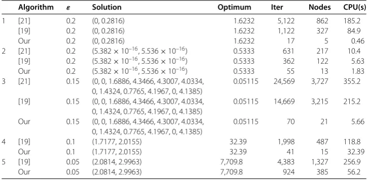
Table 1 Computational results of Examples 1-5

Algorithm ε Solution Optimum Iter Nodes CPU(s)

1 [21] 0.2 (0, 0.2816) 1.6232 5,122 862 185.2

[19] 0.2 (0, 0.2816) 1.6232 1,122 327 84.9

Our 0.2 (0, 0.2816) 1.6232 17 5 0.46

2 [21] 0.2 (5.382×10–16, 5.536×10–16) 0.5333 631 217 10.4 [19] 0.2 (5.382_×10–16_{, 5.536×10}–16_{) 0.5333 362 122 5.63} Our 0.2 (5.382×10–16_{, 5.536×10}–16_{) 0.5333 55 13 1.83} 3 [21] 0.15 (0, 0, 1.6886, 4.3466, 4.3007, 4.0334,

0, 1.4324, 0.7765, 4.1967, 0, 4.1385)

0.05115 24,569 3,727 355.2

[19] 0.15 (0, 0, 1.6886, 4.3466, 4.3007, 4.0334, 0, 1.4324, 0.7765, 4.1967, 0, 4.1385)

0.05115 14,669 3,215 215.2

Our 0.15 (0, 0, 1.6886, 4.3466, 4.3007, 4.0334, 0, 1.4324, 0.7765, 4.1967, 0, 4.1385)

0.05115 70 21 5.66

4 [19] 0.1 (1.7177, 2.0155) 32.39 1,998 487 118.8

Our 0.1 (1.7177, 2.0155) 32.39 41 15 32.39

5 [19] 0.05 (2.0814, 2.9963) 7,709.8 4,383 1,327 256.9

Our 0.05 (2.0814, 2.9963) 7,709.8 924 385 56.2

ones in [, ] by numerical examples. Because it is an approximation algorithm for solv-ing general fractional programmsolv-ing problem (P), we do not attempt comparisons with the solution methods for solving special cases of (P) (e.g., branch-and-bound [, ], outer-approximation [], cutting plane [], etc.), and the outer-approximation algorithms in [, ], which are restricted to solving problems under the quasi-concavity or low-rank assump-tions in the objective funcassump-tions. Additionally, the algorithms ([, ] and ours) are based on the exploration of a suitably defined nonuniform grid over a rectangle, but we exploit different exploration strategies to minimize the objective function over the feasible set, and use different methods to update the incumbent best value of the objective function obtained at each iteration, compared with [, ].

We implemented the three algorithms ([, ] and ours) in MATLAB b with some test experiments. Tests are run on a PC with dual processor CPU (. Hz), Intel(R), and Core(TM) i. Notice that these algorithms use different approaches for computing the lower boundliand the upper bounduiof each ratio term in the objective functions. Hence, for comparison, eachli,uiin the three algorithms is given by taking the same way (i.e., using (.)) in our computation.

Some notations in Tables , ,  have been used for column headers: Solution: the ap-proximate optimal solution; Optimum: the apap-proximate optimal value; Iter: the number of the algorithm iterations; CPU(s): the execution time in seconds; Nodes: the maximal number of the interesting grid points restored; Avg: average performance by the algorithm; Std: standard deviation of performances by the algorithm.

We first solve several sample examples, where Examples - and Examples - come from Ref. [] and Ref. [], respectively. The corresponding computational results are summarized in Table .

Example 

min–x+ x+  x– x+ 

+x– x+  –x+x+ 

Example 

min–x+ x+  x– x+ 

×x– x+  –x+x+ 

s.t. x+x≤., x≤x, ≤x≤, ≤x≤. Example 

min 

i=

ci_,x+r i

di_,x+s i

s.t. Ax≤b, x≥, where

c= (–., –., –., ., ., ., ., –., –., ., ., .), r= ,

d= (., ., –., ., ., ., –., –., ., ., ., –.), s= .,

c= (–., ., –., –., –., ., ., ., ., –., –., .), r= .,

d= (–., –., –., ., ., –., –., ., ., ., ., –.), s= ,

c= (., ., –., ., ., ., –., ., ., ., –., –.), r= .,

d= (., ., ., ., ., ., ., ., –., –., ., –.), s= .,

c= (., ., ., –., ., ., ., ., –., ., ., .), r= –.,

d= (–., ., ., –., –., ., ., –., ., –., ., –.), s= .,

c= (–., –., ., ., ., –., ., ., ., ., ., –.), r= ,

d= (., ., ., ., –., –., ., –., –., –., –., .), s= .,

c= (., –., ., ., –., –., ., –., ., –., ., –.), r= .,

d= (., ., ., ., ., –., ., –., ., –., ., .), s= .,

A= ⎡ ⎢ ⎢ ⎢ ⎢ ⎢ ⎢ ⎢ ⎢ ⎢ ⎢ ⎢ ⎢ ⎢ ⎢ ⎢ ⎢ ⎢ ⎢ ⎢ ⎢ ⎢ ⎢ ⎢ ⎢ ⎣ . . –. –. . . –. . . –. –. –. . . –. –. . –. . . –. . – . . . . . –. . . –. . –. –. . –. . . –. –. . . –. –. –. . . . –. . . . . . –. –. . . –. –. . –. –. –. . –. . –. . . . . . . –. . –. . –. –. . –. –. –. –. . –. . . –. . –. . . –. . . . –. –. . –. . –. –. . . . –. –. . –. . . . –. –. . . –. –. . . . . –. –. . –. . –. . . . –. –. . –. . –. –. . . . –. –. –. . –. –. . –. . –. . –. . –. –. –. –. . –. . . . –. –. . –. . . . . . . . . . ⎤ ⎥ ⎥ ⎥ ⎥ ⎥ ⎥ ⎥ ⎥ ⎥ ⎥ ⎥ ⎥ ⎥ ⎥ ⎥ ⎥ ⎥ ⎥ ⎥ ⎥ ⎥ ⎥ ⎥ ⎥ ⎦ ,

b= (–., –., ., ., ., ., –,

Example 

min 

i=

fi(x)

s.t. x+ x≤, ≤x≤, ≤x≤, where

f(x) = (x– )+ (x– )+ ,

f(x) = (x– )+ (x– )+ ,

f(x) = (x– )+ (x– )+ .

Example 

min 

i=

fi(x)

s.t. (x– )+ (x– )≤, ≤x≤, ≤x≤, where

f(x) = x+x,

f(x) = (x– )+ (x– ),

f(x) = (x– )+ (x– ).

Note that for solving Examples  and  we chose (l,l,l) = (, , ), (u,u,u) = (, , ) and (l,l,l) = (, , ), (u,u,u) = (, , ) which come from Ref. [], respectively. In addition, we notice that the algorithm in [] cannot be reasonable to solve Examples  and , and so we do not use it for solving them.

From Table , it can be seen easily that the proposed algorithm requires less compu-tational time for solving Examples - compared with the ones in [, ] with the same ε>  value. This is because the number of iterations and the maximal number of the in-teresting grid points restored are less than the ones in [, ] from Table , which means that the total number of the interesting grid points considered by the proposed algorithm is less than the one of the algorithms in [, ]. Also, in the three algorithms ([, ] and ours), notice that the main computational time is to check feasibility of linear programs at interesting grid points. Hence, the more interesting grid points are considered, the more computational time will be required.

Next, we apply the three algorithms ([, ] and our own) to randomly generated ex-amples as follows.

min p

i=

c_ix

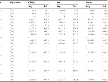
Table 2 Computational results of randomly generated test problems with (m,n) = (50, 50)

p Algorithm CPU(s) Iter Nodes

Avg Std Avg Std Avg Std

2 [21] 46.5 24.1 1,369.4 75.3 362.6 35.9

[19] 39.6 15.5 1,225.2 62.8 302.0 23.4

Our 1.2 0.5 7.8 1.6 2.2 0.5

4 [21] 5,862.1 903.8 16,973.0 994.8 3,612.5 917.2

[19] 4,590.7 802.5 17,888.1 913.8 3,294 534.1

Our 206.2 70.8 3,144.4 172.1 912.8 111.8

5 [21] 7,102.2 913.8 29,121.3 904.8 9,612.5 982.5

[19] 5,062.4 893.1 19,373.4 924.1 6,613.9 861.4

Our 813.6 113.4 5,082.9 823.7 1,403.6 813.9

6 [21] - - -

-[19] 6,384.7 895.2 38,359.4 921.7 11,869.8 938.2

Our 1,455.7 201.2 9,830.4 485.7 2,769.3 216.6

7 [21] - - -

-[19] - - -

-Our 2,754.3 430.7 12,054.4 523.5 3,257.9 433.7

8 [21] - - -

-[19] - - -

-Our 4,175.6 603.2 19,853.4 873.3 5,107.7 513.2

9 [21] - - -

-[19] - - -

-Our 6,175.1 837.9 28,251.5 869.2 8,632.2 752.3

10 [21] - - -

-[19] - - -

-Our 7,075.9 997.8 33,215.7 963.8 9,897.4 924.3

where all elements ofci∈RnandL∈Rnare random numbers generated from the interval [, ];b∈Rm_,V∈Rn_{are randomly generated vectors with all components belonging to} (, ); and each element ofA∈Rm×n_{is randomly generated in [–, ]. Nineteen examples} for selected combinations ofm(number of constraints),n(number of variables), andp

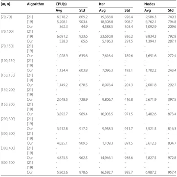
(number of linear functions in the objective function), altogether  randomly generated test instances are solved. The approximation error is fixed at ε= ., and the average computational results (standard deviation) are obtained by running the algorithms ([, ] and ours) for  times. Table  shows the numerical results for solving instances when (m,n) = (, ),pchanged in{, , , , , , , }. Similarly, asp=  and (m,n) is changed, the computational results are listed in Table . In Tables  and , ‘-’ means the problem cannot be solved within two hours.

It can be seen from Tables  and  that the proposed algorithm needs fewer iterations and interesting grid points, and so requires less computational time for solving this kind of random problems, compared with the algorithms given by [, ]. Also, it is shown by Tables  and  that the performance of the algorithms is strongly affected by changes inn

andp, specially, whenpincreases. The reason is that the number of operations required by the algorithms ([, ] and ours) is an exponential increase withpincreasing according to the corresponding computational complexity results.

Table 3 Computational results of randomly generated test problems withp= 4

[m, n] Algorithm CPU(s) Iter Nodes

Avg Std Avg Std Avg Std

[70, 70] [21] 6,518.2 869.2 19,358.8 926.4 9,586.3 749.3

[19] 5,208.1 903.4 18,308.8 908.7 6,762.1 794.8

Our 362.3 44.9 4,588.5 303.4 1,092.9 209.6

[70, 100] [21] - - -

-[19] 6,691.2 923.6 23,650.8 936.2 9,834.3 792.8

Our 528.3 65.6 5,186.3 291.5 1,394.1 287.1

[70, 150] [21] - - -

-[19] - - -

-Our 1,028.9 635.6 7,616.4 189.6 1,691.6 272.4

[100, 150] [21] - - -

-[19] - - -

-Our 1,124.4 603.8 7,096.3 193.1 1,702.2 243.4

[150, 150] [21] - - -

-[19] - - -

-Our 1,149.2 678.5 8,076.4 201.3 2,001.8 292.7

[150, 200] [21] - - -

-[19] - - -

-Our 2,048.5 728.9 9,806.7 416.8 2,671.9 397.5

[150, 300] [21] - - -

-[19] - - -

-Our 3,892.7 969.4 10,903.5 971.5 3,402.6 873.4

[200, 300] [21] - - -

-[19] - - -

-Our 3,912.8 917.2 9,938.3 911.7 3,521.5 816.3

[300, 300] [21] - - -

-[19] - - -

-Our 4,025.1 909.5 1,109.3 891.5 3,612.3 834.7

[300, 400] [21] - - -

-[19] - - -

-Our 4,875.5 962.5 14,946.1 938.6 5,827.5 972.8

[300, 500] [21] - - -

-[19] - - -

-Our 5,962.6 978.6 16,592.7 995.7 6,987.2 957.4

A comparison of the performance of the algorithms ([, ] and our own), the numerical results in Tables - show that the proposed algorithm is effective and the computational results can be obtained within a reasonable time.

5 Results and discussion

In this work, a new solution algorithm for globally solving a class of generalized fractional programming problems is presented. As further work, we think the ideas can be extended to more general type optimization problems, in which each c_i x+ci,d_i x+di in the objective function to problem (P) is replaced with a convex function, respectively.

6 Conclusion

This article proposes a new approximation algorithm for solving a class of fractional pro-gramming problems (P) without the assumptions on quasi-concavity or low-rank. In or-der to solve this problem, the original problem (P) is first converted into ap-dimensional equivalent one with a box constrained set, we then give a new approximation algorithm which can be more easily implemented compared with the ones given in [, ]. More-over, the computational complexity of such an algorithm can be derived to show that it is an FPTAS whenpis fixed, and that its computational time is an exponential increase withpincreasing. Also, the complexity results can be used as an indicator of the difficulty of some optimization problems falling into the category of (P), and so we should expect to design a more sophisticated approach where its performance is at least as good. Addi-tionally, this article not only gives a provable bound on the running time of the proposed algorithm, but also guarantees the quality of the solution obtained to problem (P).

Acknowledgements

The authors are grateful to the responsible editor and the anonymous referees for their valuable comments and suggestions, which have greatly improved the earlier version of this paper. This paper is supported by the National Natural Science Foundation of China (11671122), the Key Scientific Research Project in University of Henan Province (17A110006), and the Program for Innovative Research Team (in Science and Technology) in University of Henan Province (14IRTSTHN023).

Competing interests

The authors declare that they have no competing interests.

Authors’ contributions

PPS carried out the idea of this paper, the description of the algorithm and drafted the manuscript. TLZ completed the computation for numerical examples, and CFW carried out the analysis of computational complexity of the algorithm. All authors read and approved the final manuscript.

Publisher’s Note

Springer Nature remains neutral with regard to jurisdictional claims in published maps and institutional affiliations.

Received: 1 April 2017 Accepted: 7 June 2017

References

1. Konno, H, Gao, C, Saitoh, I: Cutting plane/tabu search algorithms for low rank concave quadratic programming problems. J. Glob. Optim.13, 225-240 (1998)

2. Henderson, JM, Quandt, RE: Microeconomic Theory: A Mathematical Approach. McGraw-Hill, New York (1971) 3. Mulvey, JM, Vanderbei, RJ, Zenios, SA: Robust optimization of large-scale systems. Oper. Res.43, 264-281 (1995) 4. Maling, K, Mueller, SH, Heller, WR: On finding most optional rectangular package plans. In: Proceedings of the 19th

Design Automation Conference, pp. 663-670 (1982)

5. Kuno, T: Polynomial algorithms for a class of minimum rank-two cost path problems. J. Glob. Optim.15, 405-417 (1999)

6. Matsui, T: NP-hardness of linear multiplicative programming and related problem. J. Glob. Optim.9, 113-119 (1996) 7. Schaible, S, Shi, J: Fractional programming: the sum-of-ratios case. Optim. Methods Softw.18, 219-229 (2003) 8. Kuno, T, Masaki, T: A practical but rigorous approach to sum-of-ratios optimization in geometric applications.

9. Teles, JP, Castro, PM, Matos, HA: Multi-parametric disaggregation technique for global optimization of polynomial programming problems. J. Glob. Optim.55, 227-251 (2013)

10. Gao, YL, Xu, CX, Yang, YJ: An outcome-space finite algorithm for solving linear multiplicative programming. Appl. Math. Comput.179, 494-505 (2006)

11. Shen, P, Wang, C: Global optimization for sum of generalized fractional functions. J. Comput. Appl. Math.214, 1-12 (2008)

12. Wang, C, Shen, P: A global optimization algorithm for linear fractional programming. Appl. Math. Comput.204, 281-287 (2008)

13. Shen, P, Yang, L, Liang, Y: Range division and contraction algorithm for a class of global optimization problems. Appl. Math. Comput.242, 116-126 (2014)

14. Shen, PP, Li, WM, Liang, YC: Branch-reduction-bound algorithm for linear sum-of-ratios fractional programs. Pac. J. Optim.11(1), 79-99 (2015)

15. Benson, HP: An outcome space branch and bound-outer approximation algorithm for convex multiplicative programming. J. Glob. Optim.15, 315-342 (1999)

16. Benson, HP, Boger, GM: Outcome-space cutting-plane algorithm for linear multiplicative programming. J. Optim. Theory Appl.104, 301-332 (2000)

17. Konno, H, Yajima, Y, Matsui, T: Parametric simplex algorithms for solving a special class of non-convex minimization problems. J. Glob. Optim.1, 65-81 (1991)

18. Liu, XJ, Umegaki, T, Yamamoto, Y: Heuristic methods for linear multiplicative programming. J. Glob. Optim.15, 433-447 (1999)

19. Locatelli, M: Approximation algorithm for a class of global optimization problems. J. Glob. Optim.55, 13-25 (2013) 20. Mittal, S, Schulz, AS: An FPTAS for optimizing a class of low-rank functions over a polytope. Math. Program.141,

103-120 (2013)

21. Depetrini, D, Locatelli, M: Approximation algorithm for linear fractional multiplicative problems. Math. Program.128, 437-443 (2011)

22. Goyal, V, Ravi, R: An FPTAS for minimizing a class of low-rank quasi-convex functions over a convex set. Oper. Res. Lett. 41, 191-196 (2013)

23. Depetrini, D, Locatelli, M: A FPTAS for a class of linear multiplicative problems. Comput. Optim. Appl.44, 276-288 (2009)

24. Goyal, V, Genc-Kaya, L, Ravi, R: An FPTAS for minimizing the product of two non-negative linear cost functions. Math. Program.126, 401-405 (2011)

25. Shen, P, Wang, C: Linear decomposition approach for a class of nonconvex programming problems. J. Inequal. Appl. 2017, 74 (2017). doi:10.1186/s13660-017-1342-y

26. Schaible, S, Ibaraki, T: Fractional programming. Eur. J. Oper. Res.12, 325-338 (1983)

27. Shen, P, Zhao, X: A fully polynomial time approximation algorithm for linear sum-of-ratios fractional program. Math. Appl.26, 355-359 (2013)

28. Hoai-Phuong, NT, Tuy, H: A unified monotonic approach to generalized linear fractional programming. J. Glob. Optim. 26, 229-259 (2003)