R E S E A R C H
Open Access
Convergence and superconvergence of
variational discretization for parabolic
bilinear optimization problems
Yuelong Tang
1*and Yuchun Hua
2*Correspondence:
[email protected] 1Institute of Computational
Mathematics, College of Science, Hunan University of Science and Engineering, Yongzhou, China Full list of author information is available at the end of the article
Abstract
In this paper, we investigate a variational discretization approximation of parabolic bilinear optimal control problems with control constraints. For the state and co-state variables, triangular linear finite element and difference methods are used for space and time discretization, respectively, superconvergence inH1-norm between the
numerical solutions and elliptic projections are derived. Although the control variable is not discrete directly, convergence of second order inL2-norm is obtained. These theoretical results are confirmed by two numerical examples.
MSC: 49J20; 65M60
Keywords: Superconvergence; Variational discretization; Bilinear optimal control
1 Introduction
It is well known that optimal control and optimization problems are approximated by many numerical methods, such as standard finite element methods (FEMs), mixed FEMs, space-time FEMs, finite volume element methods, spectral methods, multigrid methods etc.; see e.g., [5,8,10,16,17,24–26,31]. There is no doubt that FEMs occupy the most important position in these methods.
For a control constrained elliptic optimal control problem (OCP), the regularity of the control variable is lower than the regularity of the state or co-state variable. Hence, most of the researchers use piecewise constant function and piecewise linear function to ap-proximate the control variable and the state or co-state variable, respectively. If the mesh size ish, the convergent order inL2-norm for the control or inH1-norm for the state and co-state is justO(h); see e.g., [2,9,12,18]. When we use these techniques to deal with control constrained parabolic OCP, the similar convergent order isO(h+k). In order to boost the accuracy and efficiency, superconvergence and adaptive algorithm of FEMs have become research focus. The convergent order will be improved toO(h32) orO(h32+k) by superconvergence analysis. Some superconvergence results of FEMs for linear and semi-linear elliptic or parabolic OCPs can be found in [4,6,15,27–29]. Adaptive FEMs that approximate elliptic and parabolic OCPs have been investigated in [1,11,19,32] and [3], respectively.
Hinze presents a variational discretization (VD) concept for control constrained opti-mization problems in [13]. It cannot only save some computation cost but also improve
the convergent order toO(h2). Recent years, VD are used to solve different kinds of con-strained OCPs, for example, VD approximation of a convection dominated diffusion OCP with control constraints and linear parabolic OCPs with pointwise state constraints are investigated in [14] and [7], respectively.
In this paper, we consider VD approximation for constrained parabolic bilinear OCPs. The main purpose is to analyze the convergence and superconvergence. We are interested in the following control constrained parabolic bilinear OCP:
min
u∈K 1 2
T
0
y(t,x) –yd(t,x)2
+αu(t,x)2dt, (1)
yt(t,x) –div
A(x)∇y(t,x)+u(t,x)y(t,x) =f(t,x), t∈J,x∈Ω, (2)
y(t,x) = 0, t∈J,x∈∂Ω, (3)
y(0,x) =y0(x), x∈Ω, (4)
whereα> 0 represents the weight of the cost of the control,Ω∈R2is a convex bounded open set with smooth boundary ∂Ω andJ= [0,T] (0 <T < +∞). The symmetric and positive definite matrix A(x) = (aij(x))2×2 ∈[W1,∞(Ω¯)]2×2. Moreover, we assume that f(t,x)∈C(J;L2(Ω)),y
0(x)∈H01(Ω), and the set of admissible controlsKis defined by
K=v(t,x)∈L∞J;L2(Ω):a≤v(t,x)≤b, a.e. inΩ,t∈J,
where 0≤a<bare real numbers.
In this paper, we adopt the notationLs(J;Wm,q(Ω)) for the Banach space of allLs in-tegrable functions fromJinto Wm,q(Ω) with normv
Ls(J;Wm,q(Ω))= (T
0 vsWm,q(Ω)dt) 1 s
fors∈[1,∞) and the standard modification fors=∞, whereWm,q(Ω) is Sobolev spaces onΩ with norm · Wm,q(Ω) and semi-norm| · |Wm,q(Ω). We setH1
0(Ω)≡ {v∈H1(Ω) : v|∂Ω= 0}and denoteWm,2(Ω) byHm(Ω). Similarly, one can defineHl(J;Wm,q(Ω)) and
Ck(J;Wm,q(Ω)) (see e.g. [22]). In addition,corCis a generic positive constant.
The plan of our paper is as follows. In Sect.2, we present VD approximation scheme for the model problem (1)–(4). In Sect.3, we introduce some important intermediate vari-ables and their error estimates. Convergence of the control variable is derived in Sect.4. Superconvergence of the state and the co-state are established in Sect.5. In Sect.6, we present two numerical examples to illustrate our theoretical results.
2 VD approximation for parabolic bilinear OCP
In this section, we construct VD approximation for (1)–(4). We setLp(J;Wm,q(Ω)) and · Lp(J;Wm,q(Ω))byLp(Wm,q) and · Lp(Wm,q), respectively. LetW=H1
0(Ω) andU=L2(Ω). Moreover, we denote · Hm(Ω)and · L2(Ω)by · mand · , respectively. Let
a(v,w) =
Ω
(A∇v)· ∇w, ∀v,w∈W,
(f1,f2) =
Ω
f1·f2, ∀f1,f2∈U.
According to the assumptions onA, we have
We recast (1)–(4) as the following weak formulation:
min
u∈K 1 2
T
0
y–yd2+αu2
dt, (5)
(yt,w) +a(y,w) + (uy,w) = (f,w), ∀w∈W,t∈J, (6)
y(x, 0) =y0(x), ∀x∈Ω. (7)
It follows from (see e.g. [21]) that the problem (5)–(7) has at least one solution (y,u), and that if the pair (y,u)∈(H2(L2)∩L2(H1))×Kis a solution of the formulation (5)–(7), then there is a co-statep∈H2(L2)∩L2(H1) such that the triplet (y,p,u) satisfies the following optimality conditions:
(yt,w) +a(y,w) + (uy,w) = (f,w), ∀w∈W,t∈J, (8)
y(0,x) =y0(x), ∀x∈Ω, (9)
–(pt,q) +a(q,p) + (up,q) = (y–yd,q), ∀q∈W,t∈J, (10)
p(T,x) = 0, ∀x∈Ω, (11)
(αu–yp,v–u)≥0, ∀v∈K,t∈J. (12)
As in Ref. [27], we can easily prove the following lemma.
Lemma 2.1 Let(y,p,u)be the solution of(8)–(12).Then
u=min
max
a,yp
α
,b
. (13)
LetTh be regular triangulations ofΩ, such thatΩ¯ =
τ∈Thτ¯ andh=maxτ∈Th{hτ},
wherehτ is the diameter of the triangle elementτ. Furthermore, we set
Wh=
vh∈C(Ω¯) :vh|τ∈P1,∀τ∈Th,vh|∂Ω= 0
,
whereP1denotes the space of polynomials no more than order 1.
Let 0 =t0<t1<· · ·<tN =T,kn=tn–tn–1,n= 1, 2, . . . ,N,k=max1≤n≤N{kn}. Setϕn=
ϕ(x,tn) and
dtϕn=
ϕn–ϕn–1 kn
, n= 1, 2, . . . ,N.
Moreover, we define for 1≤p<∞the discrete time-dependent norms
|ϕ|lp(J;Wm,q(Ω)):=
N–l
n=1–l
knϕnpWm,q(Ω)
1 p ,
wherel= 0 for the controluand the stateyandl= 1 for the co-statep, with the standard modification forp=∞. For convenience, we denote| · |ls(J;Wm,q(Ω))by| · |ls(Wm,q)and let
Then a possible VD approximation of (1)–(4) is as follows:
min
unh∈K 1 2
N
n=1
knynh–ynd
2
+αunh2, (14)
dtynh,wh
+aynh,wh
+unhynh,wh
=fn,wh
, (15)
∀wh∈Wh,n= 1, 2, . . . ,N,
y0h(x) =yh0(x), ∀x∈Ω, (16)
whereyh0(x) =Rh(y0(x)) andRh is an elliptic projection operator which will be specified later.
Forn= 1, 2, . . . ,N, the OCP (14)–(16) again has a solution (yn
h,unh) and that if (ynh,unh)∈ Wh×Kis a solution of (14)–(16), then there is a co-statepnh–1∈Wh, such that the triplet (yn
h,pnh–1,unh)∈Wh×Wh×K, satisfies the following optimality conditions:
dtynh,wh
+aynh,wh
+unhynh,wh
=fn,wh
, ∀wh∈Wh, (17)
y0h(x) =yh0(x), ∀x∈Ω, (18)
–dtpnh,qh
+aqh,pnh–1
+unhpnh–1,qh
=ynh–ynd,qh
, ∀qh∈Wh, (19)
pNh(x) = 0, ∀x∈Ω, (20)
αunh–ynhpnh–1,vn–unh≥0, ∀v∈K. (21)
Similar to (13), the variational inequality (21) can be equivalently rewritten as follows.
Lemma 2.2 Let(yh,ph,uh)be the solution of(17)–(21).Then,for n= 1, 2, . . . ,N,we have
unh=min
max
a,y n hpnh–1
α
,b
. (22)
Remark2.1 It should be pointed out that we minimize over the infinite dimensional set Kinstead of minimizing over a finite dimensional subset ofKin (21). Then we just need to solve the discrete equations (17)–(20) and obtainuhfrom (22).
3 Error estimates of intermediate variables
Some useful intermediate variables and their important error estimates will be introduced in this section. For any control functionv∈K andwh,qh∈Wh, letynh(v),pnh(v)∈Whfor n= 1, 2, . . . ,Nsatisfy the following system:
dtynh(v),wh
+aynh(v),wh
+vnynh(v),wh
=fn,wh
, (23)
y0h(v) =yh0(x), ∀x∈Ω, (24)
–dtpnh(v),qh
+aqh,pnh–1(v)
+vnpnh–1(v),qh
=ynh(v) –ynd,qh
, (25)
pNh(v) = 0, ∀x∈Ω. (26)
We introduce the elliptic projection operatorRh:W→Wh, which satisfies: for anyφ∈ W,
a(Rhφ–φ,wh) = 0, ∀φ∈W,wh∈Wh. (27)
It has the following property (see e.g., [4]):
Rhφ–φs≤Ch2–sφ2, ∀φ∈H2(Ω),s= 0, 1. (28)
Lemma 3.1 Let(y,p,u)be the solution of(8)–(12)and(yh(u),ph(u))be the discrete solution of(23)–(26)with v=u.Suppose that u∈l2(H1)and y,p∈l2(H2)∩H2(L2)∩H1(H2),we have
yh(u) –y l2(L2)+ ph(u) –p l2(L2)≤C
h2+k. (29)
Proof Setv=uin (23), then from Eq. (8) and the elliptic projection operatorRh. Forn= 1, 2, . . . ,Nand∀wh∈Wh, we derive
dtynh(u) –dtRhyn,wh
+aynh(u) –Rhyn,wh
+unynh(u) –Rhyn
,wh
= –dtRhyn,wh
–ayn,wh
–unRhyn,wh
+fn,wh
= –dtRhyn–dtyn,wh
–dtyn–ynt,wh
–unRhyn–yn
,wh
. (30)
We note that
dtynh(u) –dtRhyn,ynh(u) –Rhyn
≥ 1 kn
ynh(u) –Rhyn2–ynh(u) –Rhynynh–1(u) –Rhyn–1 (31)
and
aynh(u) –Rhyn,ynh(u) –Rhyn
≥unynh(u) –Rhyn
,Rhyn–ynh(u)
. (32)
By choosing wh=ynh(u) –Rhynin (30) and using (31)–(32) and Hölder’s inequality, and multiplying both sides of (30) byknand summingnfrom 1 toN∗(1≤N∗≤N), we get
yNh∗(u) –RhyN
∗
≤ N∗
n=1
(Rh–I)
yn–yn–1+ N∗
n=1
yn–yn–1–knynt
+ N∗
n=1 knun
Rhyn–yn
≤ N∗
n=1
Ch2yn–yn–12+ N∗
n=1
tn
tn–1
(tn–1–t)yttdt
+C N∗
n=1
≤Ch2 N∗
n=1
tn
tn–1
yt2dt+k
N∗
n=1
tn
tn–1
yttdt+Ch2 N∗
n=1
knyn2
≤Ch2
tN∗
0
yt2dt+k
tN∗
0
yttdt+Ch2|y|l2(H2)
≤Ch2ytL2(H2)+kyttL2(L2)+h2|y|l2(H2)
. (33)
Hence
yh(u) –Rhy l∞(L2)≤C
h2+k. (34)
It follows from (28) that
|Rhy–y|2l2(L2)= N
n=1
knRhyn–yn2≤Ch4|y|2l2(H2). (35)
According to (34)–(35) and the embedding theorem, we obtain
yh(u) –y l2(L2)≤C
h2+k. (36)
Similarly, we can derive
ph(u) –p l2(L2)≤C
h2+k. (37)
Therefore, (29) follows from (36) and (37).
4 Convergence analysis
In this section, we will derive the convergence analysis for the control variable. For ease of exposition, we set
J(u) =1 2
T
0
y–yd2+αu2
dt,
Jh(uh) = 1 2
T
0
yh–yd2+αuh2
dt.
It can be shown that
J(u),v=
T
0
(αu–yp,v)dt,
Jhk (uh),v
= N
n=1 kn
αunh–ynh(uh)pnh–1(uh),v
.
In many applications, the objective functionalJ(·) is uniform convex near the solutionu (see, e.g., [23]) that is closely related to the second order sufficient conditions of the control problem. It is assumed in many studies on numerical methods of the problem (see, e.g., [2]). Hence, if handk are small enough, we can assume that Jhk(·) is uniform convex, namely, there is a positive constantc, such that
c|u–v|2l2(L2)≤
Theorem 4.1 Let(y,p,u)and(yh,ph,uh)be the solutions of(8)–(12)and(17)–(21), respec-tively.Assume that yh(u),p∈l∞(L∞)and all the conditions in Lemma3.1are valid.Then we have
|u–uh|l2(L2)≤C
h2+k. (39)
Proof Setv=uhandv=uin (12) and (21), respectively, we obtain
(αu,u–uh)≤(yp,u–uh), ∀t∈J, (40)
and
αunh–ynhpnh–1,un–unh≥0, n= 1, 2, . . . ,N. (41)
From (38) and (40)–(41), we have
c|u–uh|2l2(L2)≤
Jhk (u) –Jhk (uh),u–uh
= N
n=1 kn
αun–ynh(u)phn–1(u),un–unh
– N
n=1 kn
αunh–ynh(uh)phn–1(uh),un–unh
≤ N
n=1 kn
ynpn–ynh(u)pn,un–unh
+ N
n=1 kn
ynh(u)pn–ynh(u)pn–1,un–unh
+ N
n=1 kn
yhn(u)pn–1–ynh(u)phn–1(u),un–unh
:=I1+I2+I3. (42)
According to Young’s inequality withand Lemma3.1,I1can be estimated as follows:
I1=
N
n=1 kn
pnyn–ynh(u),un–unh
≤C() y–yh(u)
2
l2(L2)+|u–uh|2l2(L2)
≤C()h2+k2+|u–uh|2l2(L2). (43)
For the second termI2, by using Young’s inequality with, we have
I2=
N
n=1 kn
yn h(u)
pn–pn–1,un–un h
From Young’s inequality withand Lemma3.1, we get
I3=
N
n=1 kn
yhn(u)pn–1–phn–1(u),un–unh
≤C() p–ph(u)
2
l2(L2)+|u–uh|2l2(L2)
≤C()h2+k2+|u–uh|2l2(L2). (45)
Letbe small enough, then (39) follows from (42)–(45).
5 Superconvergence analysis
In this section, we will derive superconvergence of the state and co-state variables.
Theorem 5.1 Let(y,p,u)and(yh,ph,uh)be the solutions of(8)–(12)and(17)–(21), respec-tively.Assume that yh∈l∞(L∞)all the conditions in Theorem4.1hold,we have
|Rhy–yh|l2(H1)+|Rhp–ph|l2(H1)≤C
h2+k. (46)
Proof From (8) and (17), for anywh∈Whandn= 1, 2, . . . ,N, we have
ynt –dtynh,wh
+ayn–ynh,wh
+unyn–ynh,wh
=ynhunh–un,wh
. (47)
According to the definition ofRh, we get
dtRhyn–dtynh,wh
+aRhyn–ynh,wh
+unRhyn–ynh
,wh
=dtRhyn–dtyn+dtyn–ynt +un
Rhyn–yn
+ynhunh–un,wh
. (48)
Note that
dtRhyn–dtynh,Rhyn–ynh
≥ 1 2kn
Rhyn–ynh
2
–Rhyn–1–ynh–1
2
(49)
and
dtRhyn–dtyn,Rhyn–ynh
≤dtRhyn–dtynRhyn–ynh ≤Ch2dtyn2Rhyn–ynh
≤Ch2kn–1
tn
tn–1
yt2dtRhyn–ynh)
≤Ch2k– 1 2 n ytL2(t
n–1,tn;H2(Ω))Rhy n–yn
In addition
dtyn–ynt,Rhyn–ynh
=kn–1yn–yn–1–knynt,Rhyn–ynh
≤kn–1yn–yn–1–knyntRhyn–ynh
=kn–1
tn
tn–1
(tn–1–s)(ytt)(s)ds
Rhyn–ynh
≤Ck 1 2
nytt(v)L2(t
n–1,tn;L2(Ω))Rhy n–yn
h. (51)
By choosingwh=Rhyn–ynhin (48) and using (49)–(51) and Young’s inequality with, then multiplying both sides of (48) by 2knand summingnfrom 1 toN, we get
RhyN–yNh
2 +c
N
n=1
knRhyn–ynh
2 1
≤C()h4yt
2
L2(H2)+k2ytt
2
L2(L2)+h4|y|2l2(H2)+|uh–u|2l2(L2)
+
N
n=1
kRhyn–ynh
2
. (52)
From (39) and (52), we obtain
|Rhy–yh|l2(H1)≤C
h2+k. (53)
Similarly, we can prove
|Rhp–ph|l2(H1)≤C
h2+k. (54)
Hence, (46) follows from (53)–(54).
6 Numerical experiments
For an acceptable errorTol, we present the following VD approximation algorithm in which we have omitted the subscripthjust for ease of exposition.
Algorithm 6.1(VD approximation algorithm) Step 1. Initializeu0.
Step 2. Solve the following equations:
⎧ ⎪ ⎪ ⎪ ⎪ ⎪ ⎪ ⎪ ⎪ ⎨ ⎪ ⎪ ⎪ ⎪ ⎪ ⎪ ⎪ ⎪ ⎩
(yin–yin–1
k ,w) +a(yin,w) + (uniyin,w) = (fi,w), yi
n,yin–1∈Wh, ∀w∈Wh, (pin–1–pin
k ,q) +a(q,pin–1) + (uinpni–1,q) = (yin–yid,q), upi
n,pin–1∈Wh, ∀q∈Wh, un+1=min(max(a,ynαpn),b).
(55)
LetΩ = [0, 1]×[0, 1],T = 1,α= 1,a= 0,b= 1 andA(x) is a unit matrix. We solve the following two examples with AFEPack. The details can be found at [20]. We denote | · |l2(H1) and| · |l2(L2) by| · |1 and| · |, respectively. The convergence order rate: Rate= log(ei+1)–log(ei)
log(hi+1)–log(hi), whereeiandei+1 denote errors when mesh sizeh=hiandh=hi+1, respectively.
Example1 The data are as follows:
p(x,t) = (1 –t)sin(2πx1)sin(2πx2),
y(t,x) =tsin(2πx1)sin(2πx2),
u(t,x) =minmax0,y(t,x)p(t,x), 1,
f(t,x) =yt(t,x) –div
A(x)∇y(t,x)+u(t,x)y(t,x),
yd(t,x) =y(t,x) +pt(t,x) +div
A∗(x)∇p(t,x)–u(t,x)p(t,x).
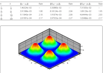
The errors based on a sequence of uniformly meshes are shown in Table1, where we can see|u–uh|=O(h2+k),|Rhy–yh|1=O(h2+k) and|Rhp–ph|1=O(h2+k). When h=801,k=6401 andt= 0.5, the numerical solutionuhis shown in Fig.1.
Example2 The data are as follows:
p(t,x) = (1 –t)x1(1 –x1)x2(1 –x2),
y(t,x) =tx1(1 –x1)x2(1 –x2),
u(t,x) =minmax0,y(t,x)p(t,x), 1,
Table 1 Numerical results of Example1
h k |u–uh| Rate |Rhy–yh|1 Rate |Rhp–ph|1 Rate
1 10
1
10 1.46324e–02 – 3.35880e–02 – 7.31505e–02 –
1 20
1
40 3.91388e–03 1.90 8.18124e–03 2.04 1.89129e–02 1.95
1 40
1
160 9.11840e–04 2.10 1.91874e–03 2.09 4.64444e–03 2.03
1 80
1
[image:10.595.117.479.464.718.2]640 2.01991e–04 2.17 3.97933e–04 2.27 1.03486e–03 2.17
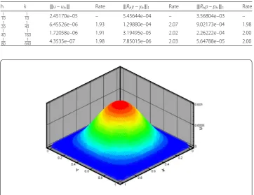
Table 2 Numerical results of Example2
h k |u–uh| Rate |Rhy–yh|1 Rate |Rhp–ph|1 Rate
1 10
1
10 2.45170e–05 – 5.45644e–04 – 3.56804e–03 –
1 20
1
40 6.45526e–06 1.93 1.29880e–04 2.07 9.02173e–04 1.98
1 40
1
160 1.72058e–06 1.91 3.19495e–05 2.02 2.26222e–04 2.00
1 80
1
[image:11.595.117.480.95.374.2]640 4.3535e–07 1.98 7.85015e–06 2.03 5.64788e–05 2.00
Figure 2The numerical solutionuhatt= 0.5, Example2
f(t,x) =yt(t,x) –div
A(x)∇y(t,x)+u(t,x)y(t,x),
yd(t,x) =y(t,x) +pt(t,x) +div
A∗(x)∇p(t,x)–u(t,x)p(t,x).
The errors|u–uh|,|Rhy–yh|1and|Rhp–ph|1on a sequence of uniformly meshes are shown in Table2. Whenh=801,k=6401 andt= 0.5, we plot the profile ofuhin Fig.2.
From the numerical results in Example1and Example2, we see that|u–uh|,|Rhy– yh|1and|Rhp–ph|1are the second order convergent. Our numerical results and theo-retical results are consistent.
7 Conclusions
Although there has been extensive research on convergence and superconvergence of FEMs for various parabolic OCPs, mostly focused on linear or semilinear parabolic cases (see, e.g., [6,10,16,26,30]), the results on convergence and superconvergence areO(h+k) andO(h32 +k), respectively. Recent years, VD are used to deal with different OCPs in [7,
13,14]. While there is little work on bilinear OCPs. Hence, our results on convergence and superconvergence of VD for bilinear parabolic OCPs are new.
Acknowledgements
The authors are very grateful to both referees for carefully reading of the paper and their comments and suggestions.
Funding
Abbreviations
FEMs, finite element methods; OCP, optimal control problem; VD, variational discretization.
Availability of data and materials
Not applicable.
Competing interests
The authors declare that they have no competing interests.
Authors’ contributions
The authors have participated in the sequence alignment and drafted the manuscript. They have approved the final manuscript.
Author details
1Institute of Computational Mathematics, College of Science, Hunan University of Science and Engineering, Yongzhou,
China.2College of Science, Hunan University of Science and Engineering, Yongzhou, China.
Publisher’s Note
Springer Nature remains neutral with regard to jurisdictional claims in published maps and institutional affiliations.
Received: 15 May 2019 Accepted: 28 August 2019 References
1. Becker, R., Kapp, H., Rannacher, R.: Adaptive finite element methods for optimal control of partial differential equations: basic concept. SIAM J. Control Optim.39(1), 113–132 (2000)
2. Casas, E., Tröltzsch, F.: Second-order necessary and sufficient optimality conditions for optimization problems and applications to control theory. SIAM J. Control Optim.13(2), 406–431 (2002)
3. Chen, T., Xiao, J., Wang, H.: Multi-mesh adaptive finite element algorithms for constrained optimal control problems governed by semi-linear parabolic equations. Acta Math. Appl. Sin. Engl. Ser.30(2), 411–428 (2014)
4. Chen, Y., Dai, Y.: Superconvergence for optimal control problems governed by semi-linear elliptic equations. J. Sci. Comput.39, 206–221 (2009)
5. Chen, Y., Huang, F.: Galerkin spectral approximation of elliptic optimal control problems withH1-norm state constraint. J. Sci. Comput.67, 65–83 (2016)
6. Dai, Y., Chen, Y.: Superconvergence for general convex optimal control problems governed by semilinear parabolic equations. ISRN Appl. Math.2014, 1–12 (2014)
7. Deckelnick, K., Hinze, M.: Variational discretization of parabolic control problems in the presence of pointwise state constraints. J. Comput. Math.29(1), 1–16 (2011)
8. Engel, M., Griebel, M.: A multigrid method for constrained optimal control problems. J. Comput. Appl. Math.235, 4368–4388 (2011)
9. Falk, R.: Approximation of a class of optimal control problems with order of convergence estimates. J. Math. Anal. Appl.44, 28–47 (1973)
10. Fu, H., Rui, H.: A priori error estimates for optimal control problems governed by transient advection-diffusion equations. J. Sci. Comput.38, 290–315 (2009)
11. Ge, L., Liu, W., Yang, D.: Adaptive finite element approximation for a constrained optimal control problems via multi-meshes. J. Sci. Comput.41, 238–255 (2009)
12. Geveci, T.: On the approximation of the solution of an optimal control problem governed by an elliptic equation. RAIRO. Anal. Numér.13, 313–328 (1979)
13. Hinze, M.: A variational discretization concept in control constrained optimization: the linear-quadratic case. Comput. Optim. Appl.30, 45–61 (2005)
14. Hinze, M., Yan, N., Zhou, Z.: Variational discretization for optimal control governed by convection dominated diffusion equations. J. Comput. Math.27(2–3), 237–253 (2009)
15. Hou, C., Chen, Y., Lu, Z.: Superconvergence property of finite element methods for parabolic optimal control problems. J. Ind. Manag. Optim.7(4), 927–945 (2011)
16. Hou, T., Chen, Y.: Superconvergence of fully discrete rectangular mixed finite element methods of parabolic control problems. J. Comput. Appl. Math.286, 79–92 (2015)
17. Hou, T., Li, L.: Superconvergence and a posteriori error estimates of splitting positive definite mixed finite element methods for elliptic optimal control problems. Appl. Math. Comput.273, 1196–1207 (2016)
18. Kröner, A., Vexler, B.: A priori error estimates for elliptic optimal control problems with a bilinear state equation. J. Comput. Appl. Math.230, 781–802 (2009)
19. Li, R., Liu, W., Ma, H., Tang, T.: Adaptive finite element approximation for distributed elliptic optimal control problems. SIAM J. Control Optim.41(5), 1321–1349 (2002)
20. Li, R., Liu, W., Yan, N.: A posteriori error estimates of recovery type for distributed convex optimal control problems. J. Sci. Comput.33, 155–182 (2007)
21. Lions, J.: Optimal Control of Systems Governed by Partial Differential Equations. Springer, Berlin (1971) 22. Lions, J., Magenes, E.: Non Homogeneous Boundary Value Problems and Applications. Springer, Berlin (1972) 23. Liu, W., Tiba, D.: Error estimates for the finite element approximation of a class of nonlinear optimal control problems.
J. Numer. Funct. Optim.22, 953–972 (2001)
24. Liu, W., Yan, N.: Adaptive Finite Element Methods for Optimal Control Governed by PDEs. Science Press, Beijing (2008) 25. Luo, X., Chen, Y., Huang, Y.: A priori error estimates of Crank–Nicolson finite volume element method for parabolic
26. Meidner, D., Vexler, B.: A priori error estimates for space-time finite element discretization of parabolic optimal control problems part II: problems with control constraints. SIAM J. Control Optim.47(3), 1301–1329 (2008)
27. Meyer, C., Rösch, A.: Superconvergence properties of optimal control problems. SIAM J. Control Optim.43(3), 970–985 (2004)
28. Strouboulis, T., Wang, D., Babuška, I.: Superconvergence of elliptic reconstructions of finite element solutions of parabolic problems in domains with piecewise smooth boundaries. Comput. Methods Appl. Mech. Eng.241(3), 128–141 (2012)
29. Tang, Y., Chen, Y.: Superconvergence analysis of fully discrete finite element methods for semilinear parabolic optimal control problems. Front. Math. China8(2), 443–464 (2013)
30. Tang, Y., Hua, Y.: Superconvergence of fully discrete finite element for parabolic control problems with integral constraints. East Asian J. Appl. Math.3(2), 138–153 (2013)
31. Vallejos, M., Borzì, A.: Multigrid optimization methods for linear and bilinear elliptic optimal control problems. Computing82, 31–52 (2008)