2018 2nd International Conference on Modeling, Simulation and Optimization Technologies and Applications (MSOTA 2018) ISBN: 978-1-60595-594-0
Spiking Neural Network on Curve Fitting
Jie-qiong YU, Wen-juan ZHANG and Lei ZHANG
*School of Physics, Northeast Normal University; and National Demonstration Center for Experimental Physics Education (Northeast Normal University), Changchun 130024, P. R. China
*Corresponding author
Keywords: Spiking Neural Network, Curve fitting, MATLAB.
Abstract. Currently, curve fitting has been widely used in data processing. Spiking Neural Network is used to provide fast and accurate curve fitting with discrete data in this paper. First, the principle of Spiking Neural Network is introduced. Second, the Spiking Neural Network for curve fitting based on the MATLAB simulation platform is established. Finally, curve fitting of a linear function and an exponential function are made. The average error values are 0 and 0.3, the results show that Spiking Neural Network can be used in curve fitting effectively.
Introduction
Curve fitting is a method of processing data that uses a continuous curve approximation or matches a set of discrete points on the plane to represent a function between coordinates. Applications of curve fitting have important theoretical and practical significance for revealing the inherent law of the data. However, the traditional methods of fitting curves have some limitations, such as polynomial fitting with low accuracy and cubic spline interpolation with high precision but long computation time. In recent years, artificial neural networks are widely used in information science, brain discipline, neuron psychology and other disciplines. Artificial neural networks[1,2](ANN) are a model that processes distributed parallel information using characteristics of biological nervous system behavior. As a third-generation artificial neural network, Spiking neural network (SNN) represents the latest research results in the field of biological neuron science and ANN. SNN with better biological properties and powerful computing capabilities can simulate a variety of neuronal signals and arbitrary continuous functions [3].
SNN
SNN is a new network proposed by Mass[4]. SNN uses the accurate time of pulse to code information, compared with the traditional way that uses firing frequency of pulses to code information. Therefore, SNN is closer to the processing mechanisms of biological information.
The Model of the Spiking Neuron
The spiking neuron is a mathematical model that is closer to the biological neurons. The traditional Sigmoid neuron model changes a real number input into a real number output signal by passing a transfer function. The essence of the model is, when the spiking neuron receives an external stimulus, its membrane potential will increase. When the membrane potential reaches the threshold, the neuron will generate a spike and send an output signal [5]. There are several common neuron models such as the integrate and fire (I&F) model, (leaky integrate and fire (LIF) model, Hodgkin-Huxley (H-H) model, spike response model (SRM) model. The I & F neuron model is used in this paper, because it can obtain better dynamic characteristics of the nervous system with comprehensive comparison and is relatively simple to implement.
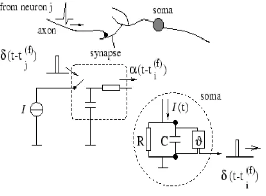
Figure 1. I&F neuron model.
The basic circuit is in a dotted circle on the right of Figure1. When the input current crosser the RC
circuit, the voltage of the capacitor (black dot) is compared with the threshold voltage , Ifu(t) at
timeti(f), an output spike ( ) ) (f i t t
will be generated. On the left side of Figure1, the spike
) (tt(jf)
generated by the presynaptic neuron will be converted to the input spike(tti(f)) of the
postsynaptic by a low-pass filter.
The basic circuit of the I&F model is composed of a capacitorCand a registerRdriven by the
currentI(t). The driven current consists of two parts. I(t)IRIC.IR is the current that crosses the
registerR, and is calculated by Ohm's LawIRu/R. Here, uis the voltage across the register.ICis the
charge current of capacitorC, which can be obtained fromCq/u and IcCdu/dt. The formula is as
follows: dt du C R t u t
I( ) ( )
(1)
Equation (1) is multiplied by R and the introduction of the integration time constant mRC, and
the standard equation can be obtained:
) ( )
(t RI t
u dt du
m
(2) The paper supposes that an I&F neuron is stimulated by a series of spikes, and the value of the reset
voltage is 0. This article assumes that a spike occurred at time tt(1). According to integral equation
(2) and initial conditions u(t(1))ur 0, we obtain the track of membrane voltage as follows:
)] exp( 1 [ ) ( ) 1 ( 0 m t t RI t u (3) If the membrane voltage is less than , no further spikes will occur. On the contrary, if the membrane voltage is more than, the spike will occur. When the spike occurs, the membrane voltage will be reset to 0, and another integral process will begin.
STDP Learning Rule
and postsynaptic neuron is adaptive. Changing the synaptic weights corresponds to the neural network. Learning rules of the first two generations of ANN do not apply to SNN[7] because of the temporal coding. The spike time dependent plasticity (STDP) rule, which evolved from the basis of the Hebb rule, is a rule of synaptic plasticity. It has a relationship with the order of firing time of two spikes [8][9], and its time-dependent theory is closer to the biological properties that are used widely in SNN. Therefore, the STDP learning algorithm is used in this paper.
[image:3.595.198.395.237.445.2]The firing time difference of connecting spiking neural is used to modify the synaptic weights in STDP[10]. As is shown in Figure 2, when the presynaptic neuron j fires before the postsynaptic neuron i, the connection strength between i and j will increase and the connection weights will increase too; Conversely, when the neuron i fires before neuron j, the connection strength between neurons will decrease and the connection weight will decrease.
Figure 2. The schematic of the STDP learning rule.
MATLAB Implementation
An SNN to curve fitting is constructed in this paper based on the spiking neurons and STDP learning rule. The network consists of a coding layer, processing layer and output layer. The information outside uses the coding layer as input, and is sent to the processing layer. The network will output results that are decoded by the output layer from the processing layer. The implementation process is as follows.
Coding Layer
The external information is transferred into a series of spikes in the coding layer. In this paper, a linear encoder is used for coding input data. As is shown in equation (4), xrepresents the input data, X
represents the range of input data, and Tmaxrepresents the maximum firing time of the spike which is defined as 20ms.
max
T
X
x
t
5
20
x
n
(5) 5 20 )(n x
d (6) 9 20 ) 2 ( x n (7) 2981 20 ) ( ) 2 (
e x
n d
(8)
Processing Layer
The sampling time is 0.01ms of the neural network in the experiment, and the time window is 20ms, creating a total of 2,000 samples. The output spike signal of the coding layer is 0.1ms, which is as wide as the input of the network in this paper. Results proved that this approach is beneficial for voltage accumulation. When the voltage accumulation reaches 1.2 volts, neurons will generate a spike, and the firing time of the spike is regarded as the result for the input signal that achieves a process changing pulse sequence in the pulse voltage signal. Meanwhile, the network weights are constantly updated based on STDP learning rule. The training times of the network are 50 times, so the network weights are updated 50 times.
Output Layer
As the input and the desired output are coded to send into the network, the actual output should be decoded to correspond with the actual input. Equation (9) is the decoding function of y = x, and equation (10) was the decoding function of y = ex.
20 5 ) ( )
(x u n
y (9) 20 2981 ) ( )
(x u n
y
(10)
Where u(n) is the firing time corresponding to the input spike, and y(x) is the actual output value corresponding to the input. Finally, the actual input and actual output will be sent as an array.
Experimental Results
The relatively simple LI&F model reflects the biological characteristics used in this paper, and the synaptic plasticity law that synaptic weights change in index form of the STDP rule is followed. The functions of the SNN are realized by fitting y = x and y = ex based on the MATLAB simulation platform.
The results of y=x are shown in Figure 3, and its actual input x=[1,3,4] are converted into n that corresponds to firing times of the spike by the information coding layer, where n=[4,12,16]. Figure
(a) The input spikes signals of network (b) The output voltage spikes signals of network
[image:5.595.83.523.67.394.2]
(c) Real output after trained and designed output (d) The error of n=2 in network
Figure 3. The result of y=x, a) the input spikes signals of the network, where I is the current, and t is time; b) the output voltage spikes signals of the network, where U is voltage; c) real output after trained and designed output, where y is
output, and x is input; d) the error of n=2 in the network, where e is error, and m are training times.
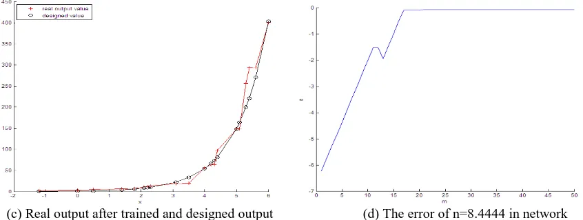
The results of y= ex are shown in Figure 4, and its actual input x=[-1.2, 0, 0.5, 1.4, 1.8, 2.1, 2.2, 2.3, 3.1, 3.5, 4, 4.2, 4.3, 4.4, 5, 5.1, 5.3, 5.4, 5.6, 6], a total of 20 values, are converted into n firing times of spikes by the information coding layer. That is, n=[1.7778, 4.4444, 5.5556, 7.5556, 8.4444, 9.1111, 9.3333, 9.5556, 11.3333, 12.2222, 13.3333, 13.7778, 14, 14.2222, 15.5556, 15.7778, 16.2222, 16.4444, 16.8889, 17.7778]. Figure 4(a) shows the input spike of the network, which is obtained from coding the real input value and also are the output spikes of presynaptic neurons. Figure 4(b) shows changes in the membrane potential of postsynaptic neurons. Figure 4(c) shows contradictions between the actual output value and the desired output value after decoding. Figure 4(d) shows the error curve of a random output in the network. As can be seen, the error will approach 0.12 after several training times.
[image:6.595.89.512.73.233.2]
(c) Real output after trained and designed output (d) The error of n=8.4444 in network
Figure 4. The result of y=ex: a) The input spikes signals of the network, where I is current, and t is time, b) the output voltage spikes signals of the network, where U is voltage, c) real output after trained and designed output, where y is
output, and x is input, and d) the error of n=8.4444 in the network, where e is error, and m are training times.
After comparing the actual output values with designed values at the end of the training, we find that the error tends to 0 and 0.3, using SNN for curving fitting of the linear function and the exponential function. It can be proved that curve fitting using SNN has the advantages of fast convergence and high accuracy.
Conclusion
Curve fitting is an important means of data processing. However, the traditional method of curve fitting has some limitations, such as polynomial fitting with low accuracy and cubic spline interpolation with high precision but long computation time. Therefore, SNN for curve fitting that is fast and accurate is used in this paper. First, the principle of the SNN is introduced in the paper. Second an SNN for curve fitting is established based on the MATLAB simulation platform. Finally, curve fitting for a linear function and exponential function is accomplished. After comparing the actual output values with designed values at the end of the training, we obtained the average error values of 0 and 0.3. The results show that the SNN has advantages of fast convergence and high accuracy on curve fitting.
Acknowledgement
This research was financially supported by the Fundamental Research Funds for the Central Universities, 2412016KJ016 and Thirteenth Five-Year Science and Technology Research Project of Education Department of Jilin Province, JJKH20170913KJ.
References
[1] Li C, Shi D, Zou Y P. 2012 Acta Phys. Sin. 61 070701 (in Chinese).
[2] Jin Q T, Wang J, Wei X L 2011 Acta Phys. Sin. 60 098701 (in Chinese).
[3] Kim J J, Diamond D M 2002 Nat. Rev. Neurosci. 3 453.
[4] Maass W. Networks of Spiking neurons: the third generation of neural network models [J]. Neural networks. 1997, (10): 1659~1671.
[5] S.M.Schuetze. The discovery of the action potenti-al. Trends Neuroscience vol.6, 1983:164-168.
[7] Kempter G, Gerstner W, Hemmen J.L. Hebbian Learning and Spiking Neurons [J]. Physical Review E. 1999, (59):4498~4514.
[8] Y. Dan, M. Poo. Spike timing-dependent plasticity of neural circuits[J]. Neuron, 2004, 44(1): 23-30.
[9] S.Song, K.D.Miller, L.F.Abbott. Competitive Hebbian learning through spike-timing-dependent synaptic plasticity[J]. Nature neuroscience, 2000, 3:919-926.