Presented at: SYNT 2018
c
Z. Liu, N. Ozay & N. Perrin This work is licensed under the Creative Commons Attribution License. Zexiang Liu Necmiye Ozay
EECS University of Michigan Ann Arbor, United States
[email protected] [email protected]
Nicolas Perrin CNRS UMR 7222, ISIR
Sorbonne Universit´e Paris, France
In this work we propose a patching algorithm to incrementally modify controllers, synthesized to satisfy a temporal logic formula, when some of the control actions become unavailable. The main idea of the proposed algorithm is to “warm-start” the synthesis process with an existing fixed-point based controller that has a larger action set. By exploiting the structure of the fixed-point based con-trollers, our algorithm avoids repeated computations while synthesizing a controller with restricted action set. Moreover, we show that the algorithm is sound and complete, that is, it provides the same guarantees as synthesizing a controller from scratch with the new action set. An example on synthe-sizing controllers for a simplified walking robot model under ground constraints is used to illustrate the approach. In this application, the ground constraints determine the action set and they might not be known a priori. Therefore it is of interest to quickly modify a controller synthesized for an uncon-strained surface, when new constraints are encountered. Our simulations indicate that the proposed approach provides at least 5-times speed-up compared to synthesizing a controller from scratch.
1
INTRODUCTION
Control synthesis techniques for discrete systems have been a central topic both for reactive synthesis and discrete-event systems [13, 14] with recent results establishing a connection between the two commu-nities [4, 15]. These techniques provide a principled means for computing a controller with correctness guarantees for systems that can either be directly modeled as or whose continuous-dynamics can be abstracted as a discrete transition system. Such discrete controllers are ubiquitous in many embedded applications.
A key challenge in control synthesis is scalability. The scalability depends both on the size of the discrete transition system and the complexity of the specification, e.g., can be doubly exponential in the length of a general linear temporal logic (LTL) specification [13]. Therefore, some research has focused on identifying fragments of LTL that have favorable complexity (see e.g., [2, 3, 17, 12]). Although these fragments lead to tractable problems, the time required for synthesis still prevents it from being applicable on-line, necessitating to consider all possible scenarios at design-time. This motivates the following questions: (i) If controllers are to be synthesized off-line for many different scenarios, and if there is a controller for a specific scenario in hand, can this controller be used to synthesize new controllers efficiently? (ii) can this modification approach be fast enough to enable on-line synthesis if new situations are encountered at run-time?
The problem of incrementally modifying an existing controller, i.e., “patching” a controller, as op-posed to re-synthesizing from scratch, has been studied for different control synthesis techniques, specif-ically in the context of robotics applications [10, 9, 18]. Livingston et al. [10] study a patching method for two player games with the specifications given by the GR(1) fragment of LTL and the control strate-gies synthesized by aµ-calculus based method. Assuming that changes in the system and environment
replace the broken part with the new one. This method is also extended to handle changes in the spec-ification such as addition of new goal regions [9]. Wong et al. [18] also consider GR(1) specspec-ifications with corresponding symbolic controller synthesis techniques and develop recovery mechanisms when the environment assumptions become invalid during execution.
This paper also considers the problem of patching controllers. Different from the existing literature mentioned above, we work with synthesis problems where there exists an explicit transition system to be controlled and the modification required is due to some of the control actions becoming unavailable. The loss of control actions is relevant in the case of actuator faults and also in the context of stabilizing a walking robot on a constrained surface, as described later, or more generally of systems with action constraints that vary with time or environment changes. Another difference is the class of specifications considered: the LTL fragment we use includes persistence requirements, which are not expressible within the GR(1) fragment, and is amenable to fixed-point based control synthesis techniques operating directly on the transition system (see e.g., [17, 12]). Our main contribution is to propose a novel controller implementation, a data structure consisting of a partially ordered set of controllers corresponding to simple fixed-points in the synthesis algorithm, that captures all the information required for modification when some of the actions become unavailable. We then present patching techniques using this data structure that modify it appropriately to compute the new controller. The proposed patching techniques are in a sense similar to warm-starting techniques in optimization, where an existing solution (not too far away from the expected new solution) is used to initialize an optimization algorithm. Similarly, we use an existing controller to initialize the synthesis algorithm for finding a controller for the new problem.
We demonstrate the proposed approach on a push recovery example for a 1D walking robot model. The potential control actions for the robot are the feasible foot placements. However, if there are ground constraints, e.g., holes, obstacles, on which the robot is not allowed to step, the available action set reduces. Such constraints might not be available a priori, hence, it is of interest to design many controllers for different sets of ground constraints. In addition, if one wants to use 1D push recovery controllers to navigate a 2D surface with constraints, it is again possible (albeit with some conservatism) to consider a large number of 1D ground constraint profiles and corresponding family of 1D controllers for the 2D navigation task. Our results for this example show that up to an order of magnitude speed-up can be achieved if the controllers for constrained surface are generated by patching the controller for the unconstrained surface.
The paper is organized as follows: In Section 2, we give the problem statement and the background knowledge about fixed-point based control synthesis. Section 3 presents the main algorithm that warm-starts a control synthesis from an existing controller, and the proof of soundness and completeness. We use a simple running example in Sections 2 and 4 to illustrate how the method works before presenting an example on control synthesis for a walking robot in Section 4 that shows the time efficiency and potential applicability of our method.
2
PRELIMINARIES
2.1 Notation
For two setsA andB, the set difference is denoted byA−B. GivenT ⊆A×B×C, for a setE ⊆A, (E,∗,∗)T refers to the set(E×B×C)∩T, and similarly forF⊆BandG⊆A×B,(∗,F,∗)T and(G,∗)T
refer to the sets(A×F×C)∩T and(G×C)∩T respectively. A listV = [x1, ...,xn]is a totally ordered
2.2 Augmented Finite Transition Systems
We consider plants modeled as augmented finite transition systems, a discrete structure that either can be used as a direct modeling tool or can be obtained by abstracting the dynamics of a continuous-control system [12].
Definition 1. An augmented finite transition system (AFTS) is a tuple T = (Q,U,→T,G,AP,hQ),
whereQis a set of states,U is a set of actions (control inputs),→T∈Q×U×Qis a transition relation
between states under specific actions,G: 2U→22Qmaps a set of actions to a set of progress groups1under that action set,APis a finite set of atomic propositions, andhQ:Q→2APis a labeling function, which
maps each state to the set of atomic propositions that evaluate to true at that state.
Without loss of generality for a given AFTS, we assume that all the actions are available at each state. Atrajectoryof an AFTST is an infinite sequence of states{s(n)}∞
n=0such that for any two
consec-utive statess(n),s(n+1)in the sequence, there exists an actiona∈Usatisfying(s(n),a,s(n+1))∈→T
and the sequence is compliant with the progress groups.
2.3 Linear Temporal Logic
Linear Temporal Logic (LTL) is utilized to describe the desired behaviors of an AFTS. It consists of logic operators (negation¬, conjunction∧, disjunction∨), and temporal operators (next, always2, eventually3and until U).
Syntax of LTL [1]: The LTL formula over a finite set of atomic propositions AP can be formed according to the grammar:
φ:=True|p|φ1∨φ2| ¬φ | φ |φ1Uφ2
wherep∈AP,φ1andφ2are also LTL formulas. The other operators can be derived as follows:φ1∧φ2= ¬(¬φ1∨ ¬φ2),φ1 =⇒ φ2=¬φ1∨φ2,3φ=TrueUφ,2φ=¬3¬φ.
Semantics of LTL[12]: Anω-word is an infinite sequence in 2AP. The satisfaction of an LTL
speci-ficationφat positioniby anω-wordw=w(0)w(1)w(2). . ., written as(w,i)|=φ, is defined inductively
as follows:
• Forφ=p∈AP,(w,i)|=piffp∈w(i)
• (w,i)|=¬φiff(w,i)6|=φ
• (w,i)|=φ1∨φ2iff(w,i)|=φ1or(w,i)|=φ2
• (w,i)|=φ iff(w,i+1)|=φ
• (w,i)|=φ1Uφ2iff∃j≥is.t.(w,j)|=φ2and(w,k)|=φ1,∀k∈[i,j)
Anω-wordwsatisfiesφif and only if(w,0)|=φ, written asw|=φ.
Given a trajectory{s(n)}∞
n=0 of an AFTS, theω-wordcorresponding to{s(n)}∞n=0is{hQ(s(n))}∞n=0,
wherehQis the labeling function of the AFTS. Given a LTL specificationφ, we say that{s(n)}∞n=0|=φ
if and only if{hQ(s(n))}∞n=0|=φ.
1A setG∈G(D)is called aprogress group under the action set D, and it is related to the following semantic notion: the
2.4 Control Synthesis and Fixed-Point Operators
The LTL specification considered in this work is of the form:
φ=2A∧32B∧ ^ i∈I
23Ri
!
(1)
for atomic propositionsA,B,Ri. Such specifications can express properties ofinvariance(2A), persis-tence(32B) andrecurrence(23Ri) . This LTL fragment, also used in [17, 12], is a subset of Gener-alized Rabin specifications [4]. As the progress groups in AFTS is equivalent to environment liveness assumptions, the formula in (1) can also be seen as a generalization of GR(1) specifications, with well-separated environments [7, 11, 15] under the well-formedness assumption in footnote 1. In what follows, with a slight abuse of notation, we treatA,B,Rias subsets of the state setQ, e.g.,A={s∈Q|A∈hQ(s)},
etc.
Roughly speaking, the control synthesis problem for an AFTS is to compute a function, i.e., control strategy, that restricts the possible actions each time a state is visited so that only the desirable trajectories of the AFTS remain. A control strategy is formally defined next.
Definition 2. Acontrol strategyfor an AFTS is a partial functionµ : (Q×U)∗×Q→2U that maps the history of state-action pairs and the current state to a set of actions.
For a given LTL specification, one can talk about the “best” control strategy in enforcing the specifi-cation and the set of initial states for which such a strategy is defined, i.e. the winning set.
Definition 3. Thewinning setfor a specificationφover an AFTST={Q,U,→T,G,AP,hQ}, written as
Wφ, is the largest subset ofQsuch that if the systemTis initially inWφ, the specification can be enforced.
Note that a control strategy as in definition 2 can require infinite memory. However for LTL specifi-cations, it is known that there exists a finite memory control strategy corresponding to the winning set. In particular, for the specifications of the form (1), we define a data structure, which we callcontroller, to implement a control strategy in a specific way. This data structure will be crucial for the patching algorithms developed in Section 3.
Definition 4. Asimple controllerfor a setD⊆Qover an AFTST={Q,U,→T,G,AP,hQ}is a function
C :D→2U, i.e. a memoryless controller that maps states inDto a set of actions.
GivenDb⊆D, a simple controllerC restricted toDbmeans that the domain ofC is restricted toD.b
Definition 5. For the AFTST={Q,U,→T,G,AP,hQ}, acontrollerC is a tuple(V,K,x), whereV is
a list of subsets ofQ,K is a list of controllers or simple controllers, which we refer to as sub-controllers ofC, andxis an internal variable that indicates the index of sub-controllers executed last time.
Overall, a controller is a tree structure with controllers at each node and simple controllers at the leaf nodes. The listK for each controller (each non-leaf node in the tree) denotes the children of that controller in the tree. Winning sets and controllers for specifications in the form of (1) are computed iteratively via fixed-point based algorithm (9) given in Appendix A.
Definition 6. Execution of controllers: In the execution time, a controllerC = (V,K,x) acts as a function that maps the current state inQto a set of feasible actions inU, for the AFTST = (Q,U,→T
,G,AP,hQ). Initially the internal variables are set to 1. Given the current state s, the output C(s) is
determined in two steps:
s
1s
2s
3s
4b
c
d
e
f
[image:5.612.214.397.69.163.2]g
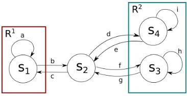
Figure 1: A simple AFTS with state space{s1,s2,s3,s4}and action space{a,b,c, ...,h}, used to illustrate how the controller works. Atomic propositions areR1={s1}andR2={s3,s4}. For simplicity, assume
no progress group exists.
– ifC results from (9), (11), (14) (see Appendix A):
x+= (
arg miny≤x{s∈V(y)}, ifx6=1
arg miny{s∈V(y)}, otherwise
– ifC results from (10) (see Appendix A):
x+= (
(x mod|K|) +1, ifs∈V(x+1) x, otherwise
wherex+refers to the value of internal variablexafter update.
(ii) Execute thex+th sub-controller and return its output:
C(s) =K(x+)(s)
In the execution ofK(x+)(s), the process above is repeated and then a sub-controller ofK(x+)is executed. Thus it is a recursive process that does not end until a simple controller is reached. The set of feasible actions are returned by that simple controller. For the sub-controllers not called in this execution, their internal variables remain unchanged.
Example 1. For a simple AFTS shown in Figure 1, given the specification φ =23R1∧23R2, the
outputs of (9) are the winning setW={s1,s2,s3,s4}, and the controllerC = (W,{C10},x=1), where its
descendant controllers2are: C0
1 = ({W,{s1},{s3,s4}},{C11,C21},x01);C11= ({{s1,s2},W,W},{C 2,0
i }3i=1,x11);
C1
2 = ({{s2,s3,s4},W,W},{Ci2,1}3i=1,x12);C 2,0
1 ={(s1,{a}),(s2,{c})};
C2,0
2 ={(s1,{a,b}),(s2,{c}),(s3,{g}),(s4,{e})};C 2,0
3 ={(s1,{a,b}),(s2,{c,d,f}),(s3,{g,h}),(s4,{e,i})};
C2,1
1 ={(s2,{d,f}),(s3,{h}),(s4,i)};C22,1={(s1,{b}),(s2,{d,f}),(s3,{g,h}),(s4,{e,i})};
C2,1
3 ={(s1,{a,b}),(s2,{c,d,f}),(s3,{g,h}),(s4,{e,i})}.
C,C10 andCi1result from (9), (10) and (11). C 2,k
i are simple controllers resulting from (13). Each
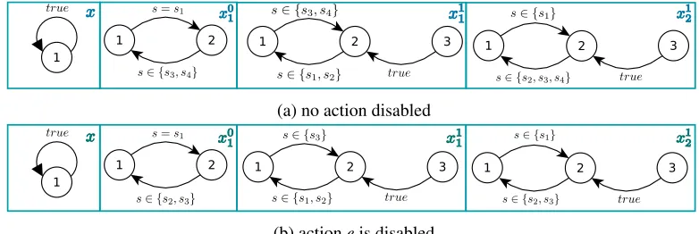
timeC is called,(x,x01,x11,x12)is updated according to Definition 6. The simple controllers inC reached at that time determines the set of feasible control inputs. The update rules for internal variables in this example 1 can be illustrated by the transition graph in Figure 2, which is consistent with Definition 6.
2In this example, in Section 4 and Appendix A, a simple controllerC
simis denoted by the set{(s,Csim(s)):s∈D}for
1
1 2 1 2 3 1 2 3
(a) no action disabled
1
1 2 1 2 3 1 2 3
[image:6.612.108.499.70.201.2](b) actioneis disabled
Figure 2: The transition graph here is a visual illustration of the update rules ofx in Definition 6. (a) corresponds to the example 1. (b) corresponds to the example in Section 4.1.sis the current state of the system in Figure 1. At each execution time, each internal variable transits from its current node to one of the neighbor node once the transition condition on the edge is satisfied. If no transition condition is satisfied, internal variable remains unchanged. Updatexfirst, and thenx0, and lastlyx10andx11.
For example, initialize the internal variables to be(1,1,1,1). Let’s start froms1and runC(s1): The
updated internal variables are(1,2,1,2), afterC(s1),C10(s1),C21(s1)andC22,1(s1)are called recursively.
The set of feasible actions is {b}=C22,1(s1). Under action b, the system in Figure 1 transits to s2. Now runC(s2). The internal variables are updated to(1,2,1,1). The set of feasible actions is{d,f}=
C2,1
1 (s2). Let’s keep doing this and always take the first action in the output ofC at each execution. The
trajectory under control ofC would be s1,s2,s4,s2,s1, ..., where the sequence of actions isb,d,e,c, ....
The trajectory visitsAandBin turn, satisfying the given specification.
2.5 Problem Statement
In this section, we formally define the problem of interest.
Problem 1. Given an AFTST= (Q,U,→T,G,AP,hQ), an LTL specificationφ=2A∧32B∧ W
i∈I23Ri
, the winning setWφ and controllerCφ, if a set of actionsUd⊆UinT is unavailable, find the new winning
set and a controller with an algorithm that exploits the knowledge ofWφ andCφ.
We start by giving an overview of our solution approach. Recall that a controller in Definition 5 has a tree structure whose nodes consist of controllers (non-leaf nodes) and simple controllers (leaf nodes): the non-leaf nodes are computed by algorithm (10), (11) and (12); the leaf nodes are computed by algorithm (13) and (14) (see Appendix A). Except for (9), each algorithm in the appendix corresponds to one underlying specification, specified by its input parameters. In Section 3, we show that each algorithm in the appendix has a corresponding patching algorithm (denoted with an over-bar on the operator for the original algorithm) which restricts an existing controller resulting from it to a smaller action space for a stronger specification3. These patching algorithms allow us to offer a solution to Problem 1 by patching the descendant controllers of a controller resulting from algorithm (9) one by one. Furthermore, since there is an order between the nodes in each layer of the tree structure (recall thatK is a list), they need to be patched in the order that they are generated.
3In general, for specifications
φ andψ, “φ is stronger thanψ” means that wheneverφis satisfied,ψ is satisfied. Here a
To get the intuition, consider a simple invariance specification (2A) and the corresponding winning setW2A computed through a simple contracting fixed-point that starts with the setA and shrinks this
set until it finds the maximal invariant set that is contained inA. In this case the controllerC2A is just
a chain (instead of an arbitrary tree) with a single simple controller. If the action set is reduced, then one can use the same simple contracting fixed-point with the new action set this time initialized with the setW2A. SinceW2A in general is smaller thanA, the new fixed point algorithm needs less iterations.
Our patching algorithm generalizes this idea to nested fixed-points where we systematically restrict the inputs to each of the algorithms recursively, using the controller data structure introduced.
3
PATCHING METHOD
Before presenting the patching methods, we state several properties of winning sets, which are vital to the success of patching existing controllers.
Given an AFTST = (Q,U,→T,G,AP,hQ)and an LTL specificationφ, compute its winning setWφ
and the winning control strategyCφ via the corresponding algorithm listed in Appendix A. Now disable
the set of actionsUd⊆Uin the AFTST, which results in a new AFTSTb= (Q,U,b → b
T,G,AP,hQ), where b
U=U−Ud and→Tb=→T −{(s1,a,s2):s1,s2∈Q,a∈Ud,(s1,a,s2)∈→T}. Re-compute the winning
set and controller , denoted byWbφ andCbφ, for a specification the same as or stronger than φ overTb via the same algorithm. Here a stronger specification always refers that input parameterZof algorithms (10), (11), (12) and (14) shrinks to a smaller setZb⊆Z(the other parameters are kept the same) afterUd
is removed from the action space. TypicallyZis the target set we want to reach, which shrinks due to the unavailable actions. Then, we have the following theorems, proofs of which are omitted for brevity:
Theorem 1. For algorithm (14), we have(Wbφ∪Zb)⊆(Wφ∪Z).
Theorem 2. For algorithms (9), (10), (11), (12) and (13), we haveWbφ ⊆Wφ.
If we fix the specification to be in the form of (1), Theorems 1 and 2 say that the winning sets of the controller and its nodes afterUd is disabled are bounded by winning sets of the controller and its nodes
beforeUd is disabled (or by the union of winning sets andZfor simpler controllers resulting from (14)),
which is the basis for our warm-starting synthesis method. Based on this fact, it is possible to search the feasible control strategies inside the existing controllers, i.e. patching the existing controllers, instead of re-synthesizing from scratch, for they contain the control strategies for a larger winning set than we need. Actually, we show that all the feasible control strategies for the new problem setting can be obtained by patching the existing controllers in the next two sections.
3.1 Patching Simple Controllers
A controller is a tree structure built on simple controllers, i.e. the leaf nodes in the tree structure. Thus we need to patch the leaf nodes firstly, and then patch their parent nodes, and so forth. In this section, we discuss the patching algorithms for the simple controllers, and then in the following section we will show how to patch the other nodes building on the leaf nodes, and the controller resulting from (9).
Definition 7. Given a simple controllerC over an AFTST = (Q,U,→T,G,AP,hQ), afinite transition system(FTS) corresponding toC isA(C) = (QC,UC,→A(C)), whereQCis the set of states that appear
in→A(C),UC={u:u∈C(s),∀s∈D},→A(C)={(s1,u,s2)∈→T:s1∈D,s2∈Q,u∈C(s1)}, andDis
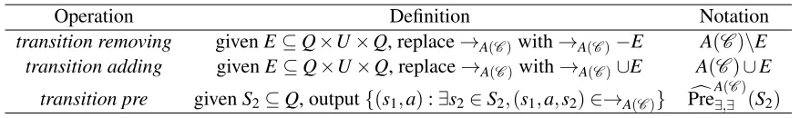
Table 1: Basic Operations on the FTS corresponding to controllerC
Operation Definition Notation
transition removing givenE⊆Q×U×Q, replace→A(C)with→A(C)−E A(C)\E transition adding givenE⊆Q×U×Q, replace→A(C)with→A(C)∪E A(C)∪E
transition pre givenS2⊆Q, output{(s1,a):∃s2∈S2,(s1,a,s2)∈→A(C)} Prec A(C)
∃,∃ (S2)
Remark1. By Definition 7,A(C)can be easily constructed from the simple controllerC and the AFTS T. Conversely,C can be constructed fromA(C) byC ={(s,D(s)):s∈W,D(s)6=/0}, whereD(s) =
{u:(s,u,s2)∈→A(C)}.
A(C)contains the transitions behind the state-action pairs inC, so that we can search invalid tran-sitions inA(C)after some actions become unavailable. Also, by Remark 1, it is easy to convert C to A(C)and vice versa. Therefore, we patch a simple controller C by modifying its corresponding FTS A(C)and then transferringA(C)toC. Several operations applied to the FTSA(C)are defined in Table 1, with which we are ready to modify simple controllers resulting from (13) and (14), i.e. PreT∃,,U∀(V)and
InvD∃,G(Z,B).
Suppose that W and C are the winning set and controller resulting from Pre∃T,,U∀(V). Given Vb=
V−∆V, we want to modifyW andC to be the winning set and controller resulting from Pre∃Tb,,∀Ub(Vb). Intuitively if we can find all the invalid transitions (s1,u,s2) inA(C) due to u∈Ud or s2∈∆V, and
remove them fromA(C), that would result in a controller that works for the new problem setting, based on which, the patching operator for (13) is:
[Wb,Cb] =Pre
T,U
∃,∀(C,∆V,Ud)
=
T0=A(C)\(∗,Ud,∗)→A(C)
E=Prec T0
∃,∃(∆V)
A(Cb) =T0\(E,∗)→T
0
b
W ={s1:∃u,∃s2s.t.(s1,u,s2)∈→A(Cb)},
(2)
whereCbis converted fromA(Cb).Wb andCbare the modified winning set and controller.
Theorem 3. Wb andCbreturned by (2) are the same as the outputs resulting from Pre b
T,Ub
∃,∀(bV)in (13).
Proof: Suppose that PreTb,Ub
∃,∀(bV) returnsWt andCt. It is enough to show that A(Cb) =A(Ct), i.e. →
A(Cb)=→A(Ct). By (13) and Definition 7, it is obvious that →A(Ct)⊆→A(C) forVb ⊆V andUb ⊆U. The transitions inS= (∗,Ud,∗)→A(C)∪(E,∗)→T0 are either under actions that may push the system to ∆V or under actions inUd, so →A(Ct) and S are disjoint. →A(Cb)=→A(C)−S. Thus→A(Ct)⊆→A(Cb). By (2), transitions in A(Cb) can only take actions inUb and transit to states inVb, which implies that
→A(
b
C)⊆→A(Ct).
Suppose thatY andC are the winning set and controller resulting from InvD∃,G(Z,B). IfD∩Ud6= /0,
the winning set is empty by the definition of progress group (see[12]). GivenZb⊆Z andDsuch that D∩Ud = /0, we want to modifyY andC to be the winning set and controller for InvD∃,G(Z,Bb ). The modified winning setYb is contained byY∪(∆Z∩G∩B). Also, Inv
D,G
∃ (Z,B) computation in (14) is a
sense and its limit is the winning set. Combining these two facts, we can warm-start the contraction algorithm in (14) withY0=Y∪(∆Z∩G∩B)instead ofQ. The patching operator is:
[Yb,Cb] =Inv
D,G
∃ (Y,C,Z,Zb)
=
Y0=Y∪(∆Z∩G∩B)
∆Y0=Q−(Y0∪Zb)
T0=A(C)∪E0
k=0
repeat:
∆Yk+1=∆Yk∪Pre∀Tk,∃,D(∆Yk)
Tk+1=Tk\(∆Yk+1,∗,∗)→Tk
Yk+1=Yk−∆Yk+1
k=k+1
until Yk=Yk−1
b
Y=Yk, [−,Cb] =Pre∃Tk,∀,D(Yb∪Zb),
(3)
where∆Z=Z−Z,b E0={(s1,a,s2)∈→T:s1∈Y0,a∈D,s2∈Q}, PreT∀k,∃,D(∆Yk) ={q1:∀u∈D,∃q2∈
∆Yk,s.t.(q1,u,q2)∈→Tk}.Ybis the modified winning set, and the controllerCbcan be computed fromTk.
In regards to the patching operator in (3), we have the following result, proof of which is given in Appendix B:
Theorem 4. YbandCbreturned by (3) are the same as the outputs resulting from Inv D,G
∃ (bZ,B)in (14).
Given a simple controller C and new synthesis settings, both (2) and (3) try to find the modified winning sets insideA(C)(orA(C)∪E0). However, if we re-synthesize the new simple controllers from
scratch, (13) and (14) start to find the winning sets in the whole AFTST, which in general needs more computation cost, demonstrated by the simulation results in Section 4. However, in the worst case, there might not be any computational gains.
3.2 Patching General Controllers
In the section we are going to patch all the non-leaf nodes, i.e the controllers resulting from (10), (11), (12), and the root node, i.e. the controller result from (9), and finally Theorem 8 shows that the patching algorithm for (9) offers a solution to the Problem 1 in Section 2.5.
Assume thatZandC = (V,K,x)are the winning set and controller resulting from PGPreT∃,∀(Z,B).
GivenZb⊆Z, we want to modifyZandC to be the winning set and controller for PGPre∃Tb,∀(Z,b B). The patching operator is:
[Zb 0,
b
C] =PGPreT∃,∀(C,Z,Zb,Ud)
=
Z0=Z, Zb0=Zb,Vb={}, Kc={}, k=1
f or D∈2U:
f or G∈G(D):
i f Ud∩D=/0 :
[Vb(k),Kc(k)] =Inv
D,G
∃ (V(k),K(k),Z0,Zb0)
else: Vb(k) =/0,Kc(k) =/0
Z0=Z0∪V(k), Zb0=Zb0∪Vb(k)
k=k+1
Remove all /0inVbandKc, Cb= (Vb,Kc,x). (4)
Theorem 5. Zb0andCbreturned by (4) are the same as outputs resulting from PGPre∃Tb,∀(Z,b B)in (12).
Proof: By theorem 4, the results of (4) remain the same if we replaceInvD∃,G(V(k),K(k),Z0,Zb0)in (4) withInvD∃,G(Zb0). After the replacement, the algorithm (4) is the same as the algorithm (12). Therefore,
Assume thatX∞andC = (V,K,x)are the winning set and controller resulting from Win
T
∃,∀(BUZ).
Assume|K|=2n, i.e. (11) converges innsteps. Then, givenZb⊆Z, to get the winning set and controller for WinTb
∃,∀(BUZb), the patching operator is:
[Xb∞,Cb] =Win
T
∃,∀,(BUZ)(C,Z,Zb,Ud)
=
X0=/0,Xb0=/0,∆X=/0, Vb={},Kc={}
k=0
repeat:
[Vb(2k+1),Kc(2k+1)] =
PreT∃,,U∀(K(2k+1),Xk−Xbk,Ud)
Ek=Z∪(B∩V(2k+1))
b
Ek=Z∪(B∩Vb(2k+1))
[Vb(2k+2),Kc(2k+2)] =
PGPreT∃,∀(K(2k+2),Ek,Ebk,Ud)
Xk+1=Z∪(B∩V(2k+1))∪V(2k+2)
b
Xk+1=Zb∪(B∩Vb(2k+1))∪Vb(2k+2)
k=k+1
until k=n orXbk=Xbk−1
whileXbk6=Xbk−1:
[Vb(2k+1),Kc(2k+1)] =
PreT∃,,U∀(K(2n−1),Xn−Xbk,Ud)
b
Ek=Z∪(B∩Vb(2k+1))
[Vb(2k+2),Kc(2k+2)] =
PGPreT∃,∀(K(2n),En,Ebk,Ud)
b
Xk+1=Zb∪(B∩Vb(2k+1))∪Vb(2k+2)
k=k+1
b
X∞=Xbk, Cb= (Vb,Kc,x).
(5)
In the algorithm (5), for k<n, we patch the(2k+1)th and(2k+2)th existing sub-controllers in K. If the winning set does not converge inn iterations, fork≥n, we duplicate the last two existing sub-controllers to the tail ofK, and patch them to enlarge the winning set until convergence.
Theorem 6. Xb∞andCbreturned by (5) are the same as outputs resulting from Win∃Tb,∀(BUZb)in (11).
Proof: Similar to the proof of Theorem 5, we can replace all thePreT∃,,U∀ andPGPreT∃,∀ terms with
PreTb,Ub
∃,∀(Xbk)andPGPre∃Tb,∀(Ebk,B). Theorem 3 and 5 guarantee that the replacements are equivalent, but
we need to verify: (i)Xbk ⊆Xk andEbk⊆Ek fork<n, and (ii)Xbk⊆XnandEbk ⊆En fork≥n. Both (i)
and (ii) can be easily checked using induction argument (with the base caseXb0⊆X0 andEb1⊆E1) and Theorem 2. After the equivalent replacements, algorithm (5) and algorithm (11) become the same. Thus
their outputs must be the same.
Assume thatWandC = (V,K,x)are the winning set and controller resulting from WinT∃,∀((BUZ)∨
2(B∧(V
i∈I3Ri)). Given thatZb⊆ZandUb⊆U, patchWandC for Win∃T,∀((BUZb)∨2(B∧( V
i∈I3Ri)).
The patching operator for (10) is:
[Wb∞,Cb] =Win
T
∃,∀(ψ)(C,Z,Zb,Ud)
=
W0=V(1),Vb=V,Kc=K
Z∞i =Z∪(B∩Ri∩PreT∃,,U∀(W0))
b
Z0i=Zb∪(B∩Ri∩Pre T,U−Ud ∃,∀ (W0))
[X0i,Kc(i)] =Win
T
∃,∀,(BUZ)(Kc(i),Z∞i,Zb0i,Ud)
b
W0=Ti∈IX0i
k=0
repeat: b
Zki+1=Zb∪(B∩Ri∩Pre T,U−Ud ∃,∀ (Wbk))
[Xi
k+1,Kc(i)] =Win T
∃,∀,(BUZ)(Kc(i),Zbki,Zbki+1,Ud)
b
Wk+1=Ti∈IXki+1
k=k+1
untilWbk=Wbk−1
b
W∞=Wbk,Cb= (Vb,Kc,x).
(6)
Theorem 7. Wb∞andCbreturned by (5) are the same as outputs resulting from WinT∃b,∀((BUZb)∨2(B∧ (V
Proof:Assume thatWtis the winning set resulting from WinT∃b,∀((BUZb)∨2(B∧( V
i∈I3Ri)). Similar
to the proof of Theorem 6, we can replace all theWinT∃,∀terms in (6) withWinTb
∃,∀(BUZbki), as long as (i) b
Z0i ⊆Zi∞and (ii)Zbk+1⊆Zbk are true. (i) is trivial. For (ii), it is enough to show thatWbk+1⊆Wbk, which
can be proven by induction. The base case: Since (i) is true, by Theorem 6, we haveX0i=WinTb
∃,∀(BUZb). ThenWb0=Ti∈IWinT∃b,∀(BUZbi0)⊆
T
i∈IWinT∃,∀(BUZ∞i ) =W0by Theorem 2. Assume thatWbk+1⊆Wbk.
ThenZbki+1⊆Zbki andWbk+1= T
i∈IWinT∃b,∀(BUZbki+1)⊆ T
i∈IWinT∃,∀(BUZbki) =Wbk. Therefore by induction
argumentWbk+1⊆Wbk, andZbk+1⊆Zbk for allk. Then (ii) is true. After the replacements, (6) and (10) are
the same except that the contraction ofWk starts from the existing winning setW instead ofQ. We can
show thatWt ⊆Wbk for all k by induction (base case: Wt ⊆W0 by Theorem 2). AlsoWt is the largest
fixed-point inQby definition. So both (6) and (10) will converge to the same fixed-pointWt.
Finally we are ready to patch the controller resulting from (9) for specification in the form of (1). Assume that W and C = (V,K,x) are the winning set and controller resulting from the oper-ator WinT∃,∀ 2A∧32B∧
V
i∈I23Ri
. Assuming that |K|=n. For patching purpose, we need some extra information: the lists of winning sets and controllers returned by PreT∃,,U∀(Vk) in (9), i.e. [V1(k),K1(k)] = Pre∃T,,∀U(Vk); the lists of winning sets and controllers returned by PGPre∃T,∀(Vk,B) in
(9), i.e. [V2(k),K2(k)] =PGPreT∃,∀(Vk,B)(k=1, ...,n) ; the controllerCInv returned by WinT∃,∀((AU/0)∨ 2(A∧3Q))in the first line of (9). To restrict action space toUb=U−Ud, the patching operator for (9)
is:
[Vb∞,Cb] =Win
T
∃,∀,(φ)(C,CInv,V1,K1,V2,K2,Ud)
= b
Vinv=Win T
∃,∀,(ψ)(CInv,/0,/0,Ud)
Restrict synthesis toVbinv
b
V0=/0,V(0) =/0,Vb={},Kc={}
k=0
repeat:
b
Zk1+1=Pre∃T,,U∀(K1(k+1),V(k)−Vbk,Ud)
b
Z2k+1=PGPreT∃,∀(K2(k+1),V(k),Vbk,Ud)
Zk+1=V1(k+1)∪V2(k+1), Zbk+1=Zbk1+1 S
b
Z2k+1
[Vbk+1,Kc(k+1)] =
WinT∃,∀,(ψ)(K(k+1),Zk+1,Zbk+1,Ud)
b
V(k+1) =Vbk+1
k=k+1
until k=n orVbk=Vbk−1
whileVbk6=Vbk−1:
b
Zk1+1=Pre∃T,,U∀(K1(n),V(n−1)−Vbk,Ud)
b
Zk2+1=PGPreT∃,∀(K2(n),V(n−1),Vbk,Ud)
b
Zk+1=Zbk1+1 S
b
Zk2+1
[Vbk+1,Kc(k+1)] =
WinT∃,∀,(ψ)(K(n),Zn,Zbk+1,Ud)
b
V(k+1) =Vbk+1
k=k+1
b
V∞=Vbk,Cb= (Vb,Kc,x).
(7)
The same as (5), the patching algorithm firstly patches the existing sub-controllers. If the winning set does not converge inniterations, the last existing controller is duplicated to the tail ofKcand patched to enlarge the winning set until it converges.
Theorem 8. Vb∞andCbreturned by (7) are the same as outputs resulting from (9) that is
WinTb
∃,∀ 2A∧32B∧ ^
i∈I
23Ri
!!
.
.
Proof: Similar to the previous proofs, we want to replace all the PreT∃,,U∀,PGPreT∃,∀ andWinT∃,∀,(Ψ)
terms in (7) withPreTb,Ub
∃,∀(bVk),PGPre∃Tb,∀(bVk,Q)andWinT∃b,∀((BUZbk+1)∨2(B∧( V
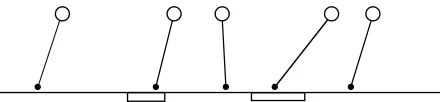
Figure 3: Simple model of one-legged 1D robots with point foot walking on a ground with holes.
(i)Vbk ⊆V(k)andZbk+1⊆Zk+1 fork<nand (ii)Vbk⊆V(n−1)andZbk+1⊆Zn fork≥n. Both (i) and
(ii) can be proven by induction using Theorems 2, 3, 5 and 7. (First prove (i) and then use the case where k=n−1 in (i) to be the base case in the induction argument for (ii)). Also, in the first line of (7) we useWinT∃,∀,(Ψ)to computeVbinv, which can can be replaced withWinT∃b,∀((AU/0)∨2(A∧3Q))since /0⊆/0.
After the replacements, (7) and (9) become exactly the same, which implies that their outputs must be
the same.
Theorem 8 shows that our patching method gives the same results as re-synthesizing from scratch via (9), and furthermore, since the algorithm (9) is sound and complete, our method is sound and complete, therefore it offers a solution to the Problem 1 stated in Section 2.5.
4
EXAMPLE
4.1 Simple Transition System
For the transition system in Figure 1, take the controller we get in Example 1 andUd ={e}as input
of the patching algorithm (7). The outputs are the modified winning setWb ={s1,s2,s3}and controller
b
C = ({Wb},{Cb10},x=1), where the descendant controllers are: b
C0
1 = ({Wb,{s1},{s2,s3}},{Cb11,Cb21},x0);Cb11= ({{s1,s2},W,W},{Cbi2,0}3i=1,x10); b
C1
2 = ({{s2,s3},W,W},{Cbi2,1}3i=1,x11);Cb12,0={(s1,{a}),(s2,{c})}; b
C2,0
2 ={(s1,{a,b}),(s2,{c}),(s3,{g})};Cb32,0={(s1,{a,b}),(s2,{c,f}),(s3,{g,h})}; b
C2,1
1 ={(s2,{f}),(s3,{h})};Cb22,1={(s1,{b}),(s2,{f}),(s3,{g,h})}; b
C2,1
3 ={(s1,{a,b}),(s2,{c,f}),(s3,{g,h})};
Let the system start froms1and initialize internal variables as(1,1,1,1). Only one trajectory is
avail-able under control ofCb, i.e.s1,s2,s3,s2,s1, ..., where the sequence of actions isb,f,g,c, ...according to the controller execution rules in Definition 6. The trajectory does not visits4, for the system is not able
to come back toAfroms4after actioneis removed.
4.2 Case study: 1D Walking Robot
We consider a model of one-legged 1D walking robot moving on a straight line, called the Linear Inverted Pendulum Model (LIPM, see [6]). This is a very simplified model of dynamics of a walking robot, but it is used by many algorithms of bipedal walking control (e.g. [5]). It consists in a point-mass robot with a massless leg moving along a line at a constant height above the ground. We do not restrict the extension of the leg nor the velocity of the leg motion (the replacement of the foot is instantaneous). The dynamics of the model are:
˙ x ˙ v
=
0 1
g/h0 0
x v
+
0
−g/h0
Table 2: The execution time of re-synthesis from scratch (row 3) and patching method (row 4) under multiple action profiles. The first row is the set of available actions. The second row is the percentage of transitions left afterUdis disabled.
Ud [1] [1 : 5] [1 : 10] [1 : 15] [1 : 20] [1 : 25] ∃trans 100% 96.57% 81.22% 60.55% 39.67% 19.00%
tsyn(s) 10.9 24.5 36.4 32.7 25.5 14.6
tpat(s) 1.3 5.7 7.7 7.3 5.9 4.8
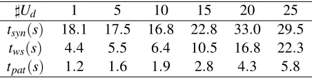
Table 3: The average execution time for re-synthesizing from scratch (row 2), re-synthesizing from the existing winning set, i.e. restrict the state space of the AFTS to be the existing winning set and re-run (9) (row 3) and our patching method (row 4) under random action profiles. The first row is number of unavailable actions (]Ud). For each number, choose 10 random sets of unavailable actions.
]Ud 1 5 10 15 20 25
tsyn(s) 18.1 17.5 16.8 22.8 33.0 29.5
tws(s) 4.4 5.5 6.4 10.5 16.8 22.3
tpat(s) 1.2 1.6 1.9 2.8 4.3 5.8
wherexis the horizontal position of the center of mass (CoM) of the robot,vis the velocity of CoM and uis the horizontal position of the foot. that the robot foot will step on.
We consider the state spaceQ= [−2.5,2.5]×[−4,4]with action spaceU= [−3.5,3.5]. Discretize QandU uniformly with grid size 0.1 and 0.2, and compute the transitions between discretized grids over-approximately using the method described in [8, 16]. Finally we get a AFTST with states indexed [1 : 4000], actions[1 : 35]and 187594 valid transitions, which is the abstraction of the walking robot.
The specification for the control synthesis is 2Q∧32B, whereB= [−2.5,2.5]×[−2,2]. It says that the CoM of the robot should always stay within[−2.5,2.5]with velocity lower than 2 after finite time from beginning. Given the specification, the winning set and controller are computed via (9) (taking A=Q,B=B,C1=Q).
Now imagine that some holes on the ground are detected, as shown in Figure 3, where the robot should avoid stepping. Therefore some actions need to be disabled. Once we determine which actions will be affected, we can put them inUdand patch the existing controllers for the new action profiles.
The experiment environment is MATLAB R2017a with CPU Intel Core i7-6820 HQ.
We choose unavailable actionsUd= [1],[1 : 5], ...,[1 : 25]for the walking robot abstraction and
com-pute the controllers via fixed-point operator (9) and the patching operator (7) respectively. The exper-iment results in Table 2 make a comparison between the time of synthesizing from scratch (tsyn) with
the time of patching existing controllers (tpat), which shows that our patching methods can shorten the
synthesis time significantly. Figure 4a shows the winning sets for eachUd, which shrink to the right part
in the state space asUd(region of holes) grows.
To further show the time efficiency, we randomly chooseUdwith sizen=1,5, ...,25. By Theorem 2,
the winning set afterUdis removed is contained by the existing one, so we can restrict the state space for
[image:13.612.192.418.252.309.2]1
1
1
1
2
2
2
2
3
3
3
3
3 4
4
4
4
4 5
5
5
5
5 6 6
6
-2 -1 0 1 2
-4 -3 -2 -1 0 1 2 3 4
W1 W2
W3
W4 W5 W
6
(a) winning set
-2 -1 0 1 2 -4
-3 -2 -1 0 1 2 3 4
(b) trajectories
0 5 10 15 20 25 30 35 time
-3 -2 -1 0 1 2 3
input
[image:14.612.141.464.69.231.2](c) inputs
Figure 4: (a) Six regions with different colors are labeled as W1,W2, ...,W6. The winning
sets under action profiles Ud = [1],[1 : 5],[1 : 10], ...,[1 : 25] are the regions corresponding to S6
i=1Wi, S6
i=2Wi, S6
i=3Wi, ..., W6 respectively. (b) Trajectories with initial state (0.85,−3.95) under
Ud = /0 (blue) and [1 : 10] (red). The region inside orange box is the target set B. (c) Inputs over
time underUd=/0 (blue) and[1 : 10](red) for trajectories in (b). The red dash-point line indicates value
corresponding to the input indexed byu=10.
in the table, the more actions are unavailable, the more time the patching algorithm needs. This can be attributed to the fact that when more actions are unavailable, the fixed point is likely to change more.
Finally, to show that formal guarantees are satisfied after patching, simulations are run for controllers before and after patching forUd = [1 : 10]. The initial state is s0=34. Figures 4b and 4c show the
trajectories and the inputs used within 60 time steps. Both trajectories go into our target region B, indicated by the orange box. The outputs from patched controller are always above the dash line where u=10, due to the unavailability of actions[1 : 10].
For practical applications in robot control, if we have the controller for the case that no constraint exists and know all the possible profiles of actions (all the possible constraints on the surface) for a known environment, the patching algorithm can generate the corresponding controllers for those action profiles very quickly.
5
CONCLUSION
In this paper, we proposed an implementation (data structure) for a controller synthesized by fixed-point based control synthesis techniques in [12]. For an existing controller with such a structure, a patching algorithm was developed to modify it for the case that some actions in the original problem setting become unavailable. Furthermore we proved that the winning set resulting from our patching algorithm was exactly the same as the winning set resulting from synthesizing a new controller from scratch.
We illustrated the efficiency of our method on a example of walking robot. The controller was synthesized for the robot described by a Linear Inverted Pendulum Model with hole constraints on the surface. We first synthesized a controller for a smooth surface without holes, and then patched it using our method for the cases that holes existed. Under the same specification, the time used by our method was only 1.4%−7% of the time used for synthesis from scratch and less than 3% on average.
subset of the original action set.
References
[1] Christel Baier & Joost-Pieter Katoen (2008):Principles of model checking. MIT press.
[2] Roderick Bloem, Barbara Jobstmann, Nir Piterman, Amir Pnueli & Yaniv Saar (2012): Synthesis of reactive (1) designs.Journal of Computer and System Sciences78(3), pp. 911–938.
[3] R¨udiger Ehlers (2011): Generalized Rabin (1) synthesis with applications to robust system synthesis. In:
NASA Formal Methods Symposium, Springer, pp. 101–115.
[4] R¨udiger Ehlers, St´ephane Lafortune, Stavros Tripakis & Moshe Y Vardi (2017): Supervisory control and reactive synthesis: a comparative introduction. Discrete Event Dynamic Systems27(2), pp. 209–260.
[5] Johannes Englsberger, Christian Ott, M´aximo A Roa, Alin Albu-Sch¨affer & Gerhard Hirzinger (2011):
Bipedal walking control based on capture point dynamics. In: Intelligent Robots and Systems (IROS),
2011 IEEE/RSJ International Conference on, IEEE, pp. 4420–4427.
[6] Shuuji Kajita, Fumio Kanehiro, Kenji Kaneko, Kazuhito Yokoi & Hirohisa Hirukawa (2001):The 3D Linear Inverted Pendulum Mode: A simple modeling for a biped walking pattern generation. In:Proceedings of the
2001 IEEE/RSJ International Conference on Intelligent Robots and Systems, pp. 239–246.
[7] Uri Klein & Amir Pnueli (2010):Revisiting synthesis of GR (1) specifications. In:Haifa Verification Confer-ence, Springer, pp. 161–181.
[8] Jun Liu & Necmiye Ozay (2014): Abstraction , Discretization , and Robustness in Temporal Logic Control of Dynamical Systems.International Conferance on Hybrid Systems: Computation and Control (HSCC), pp. 293–302, doi:10.1145/2562059.2562137.
[9] Scott C. Livingston & Richard M. Murray (2014): Hot-swapping robot task goals in reactive formal synthesis. Proceedings of the IEEE Conference on Decision and Control, pp. 101–107, doi:10.1109/CDC.2014.7039366.
[10] Scott C Livingston, Pavithra Prabhakar, Alex B Jose & Richard M Murray (2013):Patching task-level robot controllers based on a localµ-calculus formula. In:Robotics and Automation (ICRA), 2013 IEEE Interna-tional Conference on, IEEE, pp. 4588–4595.
[11] Shahar Maoz & Jan Oliver Ringert (2016):On well-separation of GR (1) specifications. In:Proceedings of
the 2016 24th ACM SIGSOFT International Symposium on Foundations of Software Engineering, ACM, pp.
362–372.
[12] Petter Nilsson, Necmiye Ozay & Jun Liu (2017): Augmented finite transition systems as abstrac-tions for control synthesis. Discrete Event Dynamic Systems: Theory and Applications 27(2), pp. 301–340, doi:10.1007/s10626-017-0243-z. Available at http://link.springer.com/10.1007/ s10626-017-0243-z.
[13] Amir Pnueli & Roni Rosner (1989):On the synthesis of a reactive module. In:Proceedings of the 16th ACM
SIGPLAN-SIGACT symposium on Principles of programming languages, ACM, pp. 179–190.
[14] Peter J Ramadge & W Murray Wonham (1987): Supervisory control of a class of discrete event processes.
SIAM journal on control and optimization25(1), pp. 206–230.
[15] Anne-Kathrin Schmuck, Thomas Moor & Rupak Majumdar (2017):On the Relation between Reactive Syn-thesis and Supervisory Control of Non-Terminating Processes. Technical Report, MPI-SWS.
[16] Fei Sun, Necmiye Ozay, Eric M Wolff, Jun Liu & Richard M Murray (2014): Efficient control synthesis for augmented finite transition systems with an application to switching protocols. In: Proceedings of the
American Control Conference, pp. 3273–3280, doi:10.1109/ACC.2014.6859428.
[V∞,C] = Win∃T,∀ 2A∧32B∧
^
i∈I
23Ri
!! =
Vinv=WinT∃,∀((AU/0)∨2(A∧3Q))
Restrict synthesis to Vinv
V0=/0,V ={},K ={},k=0
repeat:
Zk+1=PreT∃,,U∀(Vk)SPGPreT∃,∀(Vk,Q)
[Vk+1,Ck+1] =
WinT∃,∀((BUZk+1)∨2(B∧(Vi∈I3Ri)))
V(k+1) =Vk+1,K(k+1) =Ck+1
k=k+1 until Vk=Vk−1
V∞=Vk,C= (V,K,x)
(9)
[W∞,C] = WinT∃,∀((BUZ)∨2(B∧(
^
i∈I
3Ri)))
=
W0=Q,V ={},K ={}
k=0 repeat:
Zki+1=Z∪(B∩Ri∩PreT∃,,U∀(Wk))
[Xi,Ci] =WinT∃,∀(BUZki+1),∀i∈I Wk+1=
T
i∈IXi
k=k+1 until Wk=Wk−1 V(1) =Wk,
V(i+1) =B∩Ri,K(i) =Ci,∀i∈I W∞=Wk,C= (V,K,x)
(10)
[X∞,C] =WinT∃,∀(BUZ) =
X0=/0,V ={},K ={},k=0
repeat:
[Vk1,C1k] =Pre∃T,,U∀(Xk)
[Vk2,C2k] =PGPreT∃,∀(Z∪(B∩Vk1),B)
Xk+1=Z∪(B∩Vk1)∪V
2
k
V(2k+1) =Vk1,V(2k+2) =Vk2 K(2k+1) =C1k,K(2k+2) =Ck2 k=k+1
until Xk=Xk−1
X∞=Xk,C= (V,K,x)
(11)
[Z0,C] =PGPreT∃,∀(Z,B) =
Z0=Z,V ={},K ={}
k=1 f or D∈2U:
f or G∈G(D):
[Vk,Ck] =InvD
,G
∃ (Z0,B)
Z0=Z0∪Vk
V(k) =Vk,K(k) =Ck
k=k+1
C = (V,K,x)
(12)
[18] Kai Weng Wong, R¨udiger Ehlers & Hadas Kress-Gazit (2014):Correct High-level Robot Behavior in Envi-ronments with Unexpected Events.In:Robotics: Science and Systems.
A
Fixed-point Operators
In this appendix, we present algorithms from [12] to compute the winning set for a specification in the form of (1). In addition to the winning set, these algorithms provide an explicit construction of the control implementation as in Definition 5.
The most general algorithm that computes the winning set and the controller for specifications in the form of (1) is given in (9). The winning set that results from (9) is equal toV∞, i.e. the limit of the expanding sequenceVk.C is the controller corresponding to the winning setV∞.
The building blocks for algorithm (9) are (fixed-point based) operators (10), (11), (12), (13) and (14). Each operator corresponds to a type of LTL formula used in (9). Note that when a fixed-point operator appears as part of a formula, it only refers to its first output, i.e. the winning set.
The winning sets resulting from (10), (11), (14) areW∞,X∞andY∞. In words, Pre
T,U
∃,∀ is a one-step
[W,C] =PreT∃,,U∀(V) =
W={q1∈Q:∃(u∈U)∀(q2
s.t.(q1,u,q2)∈→T),q2∈V}
D(q) ={u∈U:∀(q2
s.t.(q,u,q2)∈→T),q2∈V} C={(q,D(q)):q∈Q,D(q)6=/0}
(13)
[Y∞,C] =Inv
D,G
∃ (Z,B) =
Y0= (G∩B)−Z
while Yk+16=Yk:
Yk+1=Yk∩Pre∃T,,∀D(Yk∪Z)
[−,C] =Pre∃T,,D∀(Yk∪Z)
Y∞=Yk,C restricted to Y∞
(14)
remaining indefinitely inGis impossible and thereforeZis eventually reached, which is whyY∞is part of the winning set forBUZ. On the other hand, PGPreT∃,∀(Z,B)calls Inv
D,G
∃ (Z0,B)over all the progress
groups, to collect the feasible winning states inside progress groups whereBUZcan be enforced. For controllers resulting from (9), (10), (11) and (12), their descendant controllers come from the outputs of operators they call internally. Leaf nodes in a controller always consist of simple controllers, i.e. the ones given by (13) and (14).
B
Proof of Theorem 4
Proof: Assume thatYt andCt are the winning set and controller resulting from InvD∃,G(bZ). We want to
show thatYt=Yb, which immediately impliesCt =Cb.
The winning setY of InvD∃,G(Z)is the largest subset of(G∩B)−Zsatisfying the convergence con-dition w.r.tZ, i.e. Y ⊆PreT∃,,∀D(Y∪Z)andY is the greatest fixed-point of this operator, so isYt w.r.t. Z.b Also,Yt ⊆Y0forY0in (3) by Theorem 1.
First, we showYt⊆Yb: SinceYt ⊆Y0andYk=Y0− S
i≤k∆Yi forY0,∆Yk andYk in (3), it is enough to
show∆Yk∩Yt=/0, for allk. Proceeding by induction:∆Y0∩(Yt∪Zb) = /0. Assume that∆Yk∩(Yt∪Zb) = /0, then it can be easily checked that PreTk,D
∀,∃ (∆Yk)∩Pre T,D
∃,∀(Yt∪Zb) = /0 based on the fact that→Tk⊆→T.
ForYt ⊆PreT∃,,∀D(Yt∪Zb)and∆Yk+1=∆Yk∪Pre Tk,D
∀,∃ (∆Yk),Yt∩∆Yk+1= /0. Hence by induction argument,
Yt∩∆Yk=/0 for allk, i.e.Yt⊆Yb.
Second, we showYb⊆Yt: It is enough to show thatYb satisfies the convergence condition w.r.t. Z.b By definition of Tk in (3), it is easy to check that Yk ={s1 :∃u,∃s2 s.t.(s1,u,s2)∈→Tk}. Therefore
PreTk,D
∀,∃ (∆Yk)⊆Yk for all k by definition of Pre∀Tk,,∃D in (3). Then we can express ∆Yk+1=∆Yk∪(Yk∩
PreT∀,,D∃(∆Yk)). Based on the new expression of∆Yk+1 andYk∩Zb= /0, we have∆Yk=Q−(Yk∪Zb). The limit of redefined∆Yk exists, for it is increasing and contained by a finite setQ. Once∆Yk converges,
Yk∩Pre Tk,D
∀,∃ (∆Yk)⊆∆Yk. SinceYk =Yb and ∆Yk are disjoint, we have Yb∩Pre Tk,D
∀,∃ (∆Yk) = /0, i.e. Yb∩ PreTk,D
∀,∃ (Q−(bY∪Zb)) = /0. This being empty set is equivalent to∀s1∈Yb, not (∀u∈D,∃s2∈Q−(bY∪ b
Z),(s1,u,s2)∈→T), i.e. ∀s1∈Yb,∃u∈D,∀s2∈Q−(bY∪Zb),(s1,u,s2)6∈→Tk. That implies that∀s1∈
b
Y,∃u∈D,∀(s2s.t.(s1,u,s2)→Tk),s2∈(bY∪Zb). By definition ofTk in (3), for alls1∈Yb andu∈D, if (s1,u,s2)∈→T,(s1,u,s2)∈→Tk. So we have∀s1∈Yb,∃u∈D,∀(s2s.t.(s1,u,s2)→T),s2∈(bY∪Zb), that
isYb⊆Pre T,D
![Figure 4:(a) Six regions with different colors are labeled asUsets under action profiles W1,W2,...,W6.The winning Ud = [1],[1 : 5],[1 : 10],...,[1 : 25] are the regions corresponding to�6i=1Wi, �6i=2Wi,�6i=3Wi,..., W6 respectively](https://thumb-us.123doks.com/thumbv2/123dok_us/185883.1017196/14.612.141.464.69.231/figure-regions-different-labeled-proles-regions-corresponding-respectively.webp)
