R E S E A R C H
Open Access
A weighted denoising method based
on Bregman iterative regularization
and gradient projection algorithms
Beilei Tong
**Correspondence: [email protected]
School of Mathematical Sciences, University of Science and Technology of China, Hefei, Anhui 230026, P.R. China
School of Science, Southwest University of Science and Technology, Mianyang, Sichuan 621010, P.R. China
Abstract
A weighted Bregman-Gradient Projection denoising method, based on the Bregman iterative regularization (BIR) method and Chambolle’s Gradient Projection method (or dual denoising method) is established. Some applications to image denoising on a 1-dimensional curve, 2-dimensional gray image and 3-dimensional color image are presented.
Compared with the main results of the literatures, the present numerical results of the proposed method are improved.
MSC: 65F22; 68U10; 35A15; 65K10; 52A41
Keywords: total variation; optimization; image denoising; Bregman distance; gradient projection method
1 Introduction
In this paper, we consider the image denoising problems. The objective is to find the un-known true imageu∈Rnfrom an observed imageg∈Rnformed as the follows:
g=u+n, (.)
wheren∈Rnrefers to the additive white gaussian noise. To remove the additive white gaussian noise well, Rudin, Osher and Fatemi (ROF) first proposed the total-variation (TV) regularization denoising model in []. This denoising model is actually the optimiza-tion of the ROF funcoptimiza-tional:
min
u ∇u+
λu–g
, (.)
where, for the continuous case,i.e.u∈L(),is an open subset ofRn. Here, ·
denotes
theL norm. We also denote∇u byTV(u). The TV regularization model had been
popular from then on for it can preserve the edges and the details as denoising [, ]. There are various excellent algorithms to solve the ROF denoising model [–]. In this paper, we consider two state-of-the-art denoising methods,i.e. Chambolle’s gradient pro-jection denoising algorithm [] and Osheret al.’s Bregman iterative regularization method
[]. Chambolle solved the ROF model in the dual field. The Bregman iterative regulariza-tion method in [] gave a significant improvement over standard ROF models by taking back useful information to the denoising results. Yinet al. proved a more simple equiv-alent formation to the Bregman iterative regularization model in []. It is known from the numerical examples of [] that the Bregman iterative regularization method can keep the horizontal and the vertical edges well and the bent edges badly. On the contrary, we see that Chambolle’s dual denoising method in [] can keep the curve well and the hor-izontal and the vertical edges badly. Accordingly, in this paper, we give a comprehensive denoising method based on the dual denoising algorithm [] and the Bregman iterative regularization method [, ]. In this paper, implicitly assumed, dual denoising just refers to Chambolle’s dual denoising algorithm or the gradient projection method.
Firstly, we choose a proper weight parameter β and modify the ROF functional to a modified form with a weighted taking-back-noise term:
bk+= (g+bk) +βπλK(g+bk).
The weight parameterβ∈(, ), maintains a balance between the Bregman iterative reg-ularization method and the dual denoising method. The value ofβvaries according to the noise level and it is approximately inversely proportional to the noise level. Specially, when
β= , we solve the ROF model by the gradient projection method for there is no informa-tion that is taken back to the model. As forβ= , the model becomes the Bregman iterative regularization model. Secondly, we iteratively solve the modified ROF model until the end condition is met. When <β< , we solve the modified ROF model by Chambolle’s dual algorithm. The results of the numerical experiments demonstrate that the new method cannot only restore more straight edges than the dual denosing method but also restore more bent edges than the Bregman iterative regularization method.
The rest of this paper is organized as follows. In Section , we briefly review the dual denoising method and Bregman iteration denoising method. In Section , we propose our weighted gradient projection denoising method. Then, in Section , we apply our new method to -D curve, -D gray image and -D color image denoising examples, respec-tively, and present the numerical results. Finally, we give a conclusion.
2 Preliminaries
2.1 Dual denoising method Noticing that
TV(u) =sup v∈K
(u,v)X (.)
(.) can be rewritten as
min u J(u) +
λu–g
. (.)
The Euler equation for (.) is
which is equivalent to
(u–g)/λ∈∂J(u) and equivalent to
u∈∂J∗(g–u)/λ.
The above equation can be rewritten as
∈g–u
λ –
g
λ+
λ∂J
∗g–u
λ
, (.)
whereJ∗is the Legendre-Fenchel transform ofJ[–], defined by
J∗(v) =sup u
(u,v)X–J(u). (.)
Proposition .
J∗(v) =χ κ=
if v∈κ,
+∞ otherewise. (.) Letω= (u–g)/λ, (.) is the Euler equation for the minimization problem
min ω
ω– (g/λ)
λ +
λJ
∗(ω).
By Proposition ., we getω=πK(g/λ). The solution of equation (.) can be simplified as
u=g–πλK(g). (.)
For computingu, we just need to compute the nonlinear projectionπλK(g),i.e. to solve the following problem:
minλdivp–g):∀p∈Y,|pi,j|– ≤,i= , . . . ,M,j= , . . . ,N , (.)
here,M,Nrepresent the total number of pixels in each row and in each column.
Given λ=λ> , <τ < ,p= , for anyn≥, Chambolle’s gradient projection
method for the denoising problem (.) is described as below.
forn= , . . . ,Lout
Initialization:p= ; fort= , . . . ,Lin
pn+i,j =p
n
i,j+τ(∇(divpn–g/λt))i,j
+τ|(∇(divpn–g/λ t))i,j|
;
vn+=πλt(g) =λtdivp n+;
end
λt=
Nσ
fn+ λt;
end
λt+=λt;
u=g–vn+
i.e. u=g–πλt+K(g)
.
Here Iout,Iin denote the iterative numbers of the external iterations and the internal
iterations time foru.Nis the total number of pixels.σis the noise standard deviation. For convenience, we set the inner loop timesLinand the outside loop timeIout.
Lemma .([]) Let <τ<and p= ,then,for anyλ> ,λdivpnconverges toπλnK(g)
as n→+∞.
2.2 Bregman iterative regularization denoising method
Osheret al. proposed a Bregman iterative regularization denoising method and proved the convergence []. A simple and equivalent iterative procedure to the BRI denoising model was given in [], and the convergence of this simplified method was also analyzed. Here we consider the simplified BRI denoising model in []. The simplified BIR denoising model is as follows:
uk+=artmin u∈BV()
|u|BV+μg+bk–uL , (.)
whereBV() denotes the space of functions with bounded variation onand| · |BV
de-notes the BV seminorm, formally given by
|u|BV=
|u|,
which is also referred to as the total variation (TV) of u, and update
bk+=bk+g–uk+, (.)
wherebkis the information taken back (we setb= ),gis the degenerative image
con-taminated by additive white gaussian noise.
The Bregman iteration technique has the advantage of converging quickly when applied to certain types of objective functions and the advantage of keeping a fixed value ofλas denoisings [].
Lemma .([]) Suppose that some iterate,u∗,satisfies Au∗=b.Then u∗is a solution to the constrained problem(.).
3 A weighted denoising method
of [] and [], we see that the bent parts of the curve do not get restored perfectly by the BIR method, while the straight edges are not be kept well by Chambolle’s dual denoising method. So we plan to combine these two methods to improve the restored efficiency of the noisy images. We found that the denoising effects were not very good if we just put these two methods together. This is because too much noise was taken back if the noise level is heavy. So we propose a weighted coefficient strategy to eliminate this phenomenon.
Firstly, we use the simplified Bregman iterative regularization model:
uk+=artmin u∈BV()
|u|BV+μg+bk–uL ;
for the sake of consistency, setting the parameterμin the above functional equal toλ we consider the modified ROF model
uk+=artmin u∈BV()
|u|BV+
λg+bk–u L
; (.)
if we apply Chambolle’s dual algorithm to each iteration of (.) by Chambolle’s dual algo-rithm, we have
uk+=g+bk–πλK(g+bk);
and the update
bk+=bk+ (bk+g–uk+).
By a simple derivation, we have
bk+=bk+πλK(g+bk), (.)
whereb= .
Bregman-gradient projection method initialize:
Initialization:u=g, b= , λ=λ (here, we choose aλ> )
Whileuk–uk–>tol (tolis the tolerance)
fork= , . . . ,K∗:
Using Chambolle’s dual method to computeuk+in (.), we obtain
uk+= (g+bk) –πλK(g+bk)
end
and using the new update (.):
bk+=bk+πλK(g+bk)
end
outside recycling. It is easy to see that we just need to replacegin (.) byg+bk. This mixed
denoising method is mainly based on the Bregman iterative regularization denoising and Chambolle’s gradient projection denoising method, which ensures that each sub-problem has a closed-form solution. However, if we just put these two methods together, the de-noising effects were not very good.
Secondly, we add a weight factorβ before the taking-back-noise term of the updating iteration step,i.e.
bk+=bk+βπλK(g+bk). (.)
Here, the weighted coefficientβ∈[, ],β≥, is used to balance the amount of the noises taken back to the latest denoised result. The strategy is that the bigger the noise level, the smaller theβis. This is because too much noise was taken back if the noise level is heavy. Next, we will give the mixed denoising method of BIR denoising and the dual denoising method.
Weighted Bregman-gradient projection method
Initialization:u=g, b= , λ=λ (here, we choose aλ> )
Whileuk–uk–>tol
fork= , . . . ,K∗:
Using Chambolle’s dual method to computeuk+in (.), we obtain
uk+= (g+bk) –πλK(g+bk)
end
and using the new update (.):
bk+=bk+βπλK(g+bk)
[image:6.595.117.478.535.736.2]end
Table 1 Values of the parameterβ
Dimension 1-D 2-D 3-D
σ= 12 σ= 25
β 0.4 0.1 0.1 0.05
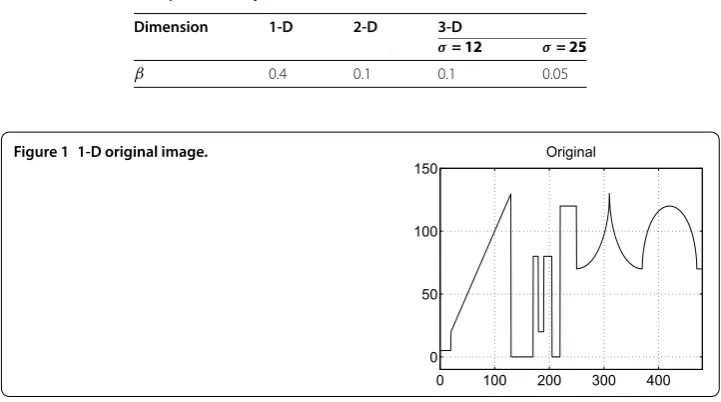
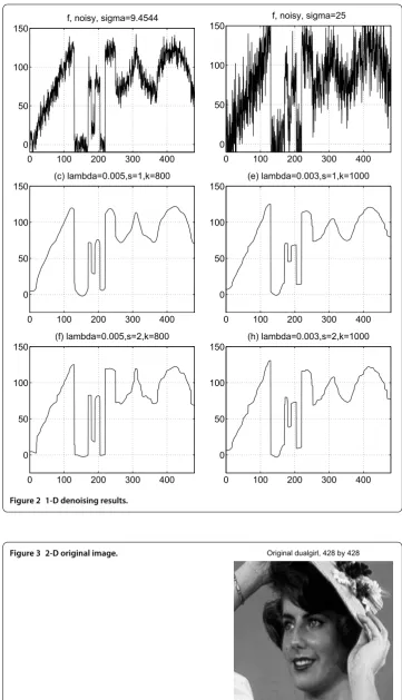
Figure 2 1-D denoising results.
Figure 4 2-D denoising results.
Figure 5 3-D original image.
those of the dual algorithms. The results presented in this paper extend and improve the related results of [] and []. The details of the parameterβare showed in Table .
4 Numerical experiments and discussions
In this section, we will examine the effectiveness of the weighted Bregman method on TV denoising. The new method was implemented in FORTRAN and MATLAB, and compiled on a Win platform.
Firstly, we test our method by denoising three kinds of images: the -D curves, the -D gray images and the -D color images.
Next, we will compare the peak signal-to-noise ratios (PSNRs) of the dual denoising method and our new denoising method. Under the same number of iterations, all the results show that the PSNRs of the new method are higher than those of the dual denoising method. Here, the PSNR is defined as follows: given a noise-freem-by-nimageIand its noisy approximationK,
PSNR= ·log
MAXI MSE
,
where the mean squared error (MSE) is defined as
MSE=
mn
m–
i= n–
j=
I(i,j) –K(i,j),
whereMAXIdenotes the maximum possible pixel value of the image. When the pixels are
represented using bits per sample,MAXIis .
Figure 6 3-D Denoising results.
Table 2 PSNR results of Chambolle’s dual method and our new method
Dimension σ Dual (dB) Ours (dB)
1-D σ= 9.4544 36.3555 40.1584
σ= 25 31.1127 32.8930
2-D σ= 12 33.9067 34.3631
σ= 25 31.1647 31.2651
3-D σ= 12 32.1209 32.7622
σ= 25 28.7921 29.6473
the dual method. Here, ‘s– ’ is the taking-back-noises iteration time and ‘k’ refers to the dual iteration number. The dual iterations stop when the infinite module of the denoised results of thekth step and (k+ )th step is less than ..
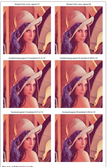
Example In the second example, we further test the effectiveness of the proposed method by denoising the gray images. The clean -D gray image of Figure is contam-inated by gaussian white noise with standard deviation and , and the noisy images are shown in the first row of Figure from left to right. A comparison of the denoising results for the dual method and the proposed method is provided in the last two rows of Figure . In the middle row of Figure , the PSNRs for the dual method are . dB (left) and . dB (right). The bottom images are the restored images using the pro-posed method, with PSNRs . dB (left) and . dB (right). The denoising pa-rameter ofAfrom left to right is . and .. Also here, the symbolkrefers to the dual iteration number. All the taking-back-noises iteration numbers are one. Comparison results show again that the contours and the details such as the girl’s hair, mole, nose and teeth are recovered more clearly by our new method than the dual method.
Example In this experiment, we come to deal with -D color image. The original RGB
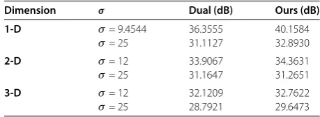
‘Lena’ image in Figure is distorted by gaussian white noises with standard deviation of and , respectively. The noisy images are shown in the Figure at the top left and the top right. In Figure , the second row, the denoised results for the dual method are shown, the PSNR of the left one is . dB and the right one is . dB. In the third row, the restoration results by the proposed method are displayed, with the PSNRs . dB (left) and . dB (right) severally. The denoising parameter ofλfrom left to right is . and ., the taking-back-noises iteration number equals one and the dual iteration numberkis ten. It is clear that, no matter the noise level is light or heavy, the restored results by our method are much better than those by the dual method, especially in the contours and details, such as the hair and the hat.
In Table , we present the PSNRs of the dual algorithm and our new method. Hereσis the noise standard deviation.
5 Conclusions
Acknowledgements
The author was supported by the Grant No. 17ZB0447 of the Scientific Research Fund of Sichuan Provincial Education Department. Also, this work was partly support by the State Key Laboratory of Science and Engineering Computing of the Chinese Academy of Sciences (LSEC of CAS). I would like to thank Dr. Chong Chen (LSEC of CAS) for his friendly inviting me to visit LSEC of CAS, and I would like to thank Prof. Gang Li (QDU) and Prof. Kelong Zhen (SWUST) for their help too.
Competing interests
The author declares that she has no competing interests.
Authors’ contributions
The author of the manuscript has read and agreed to its content and is accountable for all aspects of the accuracy and integrity of the manuscript.
Publisher’s Note
Springer Nature remains neutral with regard to jurisdictional claims in published maps and institutional affiliations.
Received: 16 September 2017 Accepted: 12 October 2017 References
1. Rudin, LI, Osher, S, Fatemi, E: Nonlinear total variation based noise removal algorithms. Phys. D, Nonlinear Phenom.
60(1-4), 259-268 (1992)
2. Aubert, G, Kornprobst, P: Mathematical Problems in Image Processing: Partial Differential Equations and the Calculus of Variations. Springer, Berlin (2002)
3. Chan, T, Shen, J: Image Processing and Analysis: Variational, PDE, Wavelet, and Stochastic Methods. SIAM, Philadelphia (2005)
4. Chambolle, A: An algorithm for total variation minimization and applications. J. Math. Imaging Vis.20(1), 89-97 (2004) 5. Osher, S, Burger, M, Goldfarb, D, Xu, J, Yin, W: An iterated regularization method for total variation-based image
restoration. In: IEEE International Conference on Imaging Systems and Techniques, pp. 170-175 (2011) 6. Yin, W, Osher, S, Goldfarb, D, Darbon, J: Bregman iterative algorithms forl1-minimization with applications to
compressed sensing. SIAM J. Imaging Sci.1(1), 143-168 (2008)
7. Chang, Q, Chern, IL: Acceleration methods for total variation-based image denoising. SIAM J. Sci. Comput.25, 982-994 (2003)
8. Goldstein, T, Osher, S: The split Bregman method for L1 regularized problems. SIAM J. Imaging Sci.2(2), 323-343 (2009)
9. Jia, R, Zhao, H: A fast algorithm for the total variation model of image denoising. Adv. Comput. Math.33(2), 231-241 (2010)