Approximations to inverse tangent function

R E S E A R C H

Open Access

Approximations to inverse tangent

function

Quan-Xi Qiao

_{and Chao-Ping Chen}

*_{Correspondence:}

chenchaoping@sohu.com

1_{School of Mathematics and}

Informatics, Henan Polytechnic University, Jiaozuo, China

Abstract

In this paper, we present a sharp Shafer-type inequality for the inverse tangent function. Based on the Padé approximation method, we give approximations to the inverse tangent function. Based on the obtained result, we establish new bounds for arctanx.

MSC: 26D05

Keywords: Inverse trigonometric function; Inequality; Approximation

1 Introduction

In 1966, Shafer [1] posed, as a problem, the following inequality:

3x

1 + 2√1 +x2 <arctanx, x> 0. (1.1) Three proofs of it were later given in [2]. Shafer’s inequality (1.1) was sharpened and gen-eralized by Qiet al.in [3]. A survey and expository of some old and new inequalities as-sociated with trigonometric functions can be found in [4]. Chenet al.[5] presented a new method to sharpen bounds of bothsincxandarcsinxfunctions, and the inequalities in exponential form as well.

For eacha> 0, Chen and Cheung [6] determined the largest numberband the smallest numbercsuch that the inequalities

bx

1 +a√1 +x2 ≤arctanx≤ cx

1 +a√1 +x2 (1.2)

are valid for allx≥0. More precisely, these author proved that the largest numberband the smallest numbercrequired by inequality (1.2) are

when 0 <a≤π

2, b=

π

2a, c= 1 +a;

when π 2 <a≤

2

π– 2, b=

4(a2_{– 1)}

a2 , c= 1 +a;

when 2

π– 2<a< 2, b=

4(a2_{– 1)}

a2 , c=

π

2a;

when 2≤a<∞, b= 1 +a, c=π 2a.

In 1974, Shafer [7] indicated several elementary quadratic approximations of selected functions without proof. Subsequently, Shafer [8] established these results as analytic in-equalities. For example, Shafer [8] proved that, forx> 0,

8x

3 +

25 +80₃x2

<arctanx. (1.3)

The inequality (1.3) can also be found in [9]. The inequality (1.3) is an improvement of the inequality (1.1).

Zhu [10] developed (1.3) to produce a symmetric double inequality. More precisely, the author proved that, forx> 0,

8x

3 +

25 +80₃x2

<arctanx< 8x 3 +

25 +256_π2x2

, (1.4)

where the constants 80/3 and 256/π2_{are the best possible.}

Remark1.1 Forx> 0, the following symmetric double inequality holds:

8x

3 +

25 +80₃x2

<arctanx<

2√15π 3 x

3 +

25 +80₃x2

, (1.5)

where the constants 8 and 2√15π

3 are the best possible. We here point out that, forx> 0, the upper bound in (1.4) is better than the upper bound in (1.5).

Based on the following power series expansion:

arctanx

3 +

25 +80 3 x

2

= 8x+ 32 4725x

7_– 64 4725x

9₊ 25,376 1,299,375x

11_{–· · ·,}

Sun and Chen [11] presented a new upper bound and proved that, forx> 0,

arctanx< 8x+ 32 4725x

7

3 +

25 +80₃x2

. (1.6)

Moreover, these authors pointed out that, for 0 <x<x0= 1.4243 . . . , the upper bound in (1.6) is better than the upper bound in (1.4). In fact, we have the following approximation formulas near the origin:

arctanx– 8x 3 +

25 +256_π2x2

=Ox3,

arctanx– 3x

1 + 2√1 +x2=O

x5,

arctanx– 8x 3 +

25 +80₃x2

and

arctanx– 8x+ 32 4725x

7

3 +

25 +80₃x2

=Ox9.

Nishizawa [12] proved that, forx> 0,

π2_x

4 +(π2_{– 4)}2_{+ (2πx)}2 <arctanx<

π2_x

4 +32 + (2πx)2, (1.7)

where the constants (π2– 4)2and 32 are the best possible.

Using the Maple software, we derive the following asymptotic formulas in theAppendix:

arctanx

x =

π2

4 +32 + (2πx)2 – 12 –π2

3π2_x4 +O

1

x5

, (1.8)

arctanx

x =

3π2

24 –π2_{+432 – 24π}2_+π4_{– 12π(12 –π}2_{)x+ (6πx)}2

+π 4_{– 72}

18π3_x5 +O

1

x6

, (1.9)

and

x

π

2 –arctanx

=x 2₊ 4

15 x2₊3 5

+O

1

x6

(1.10)

asx→ ∞.

In this paper, motivated by (1.9), we establish a symmetric double inequality forarctanx. Based on the Padé approximation method, we develop the approximation formula (1.10) to produce a general result. More precisely, we determine the coefficientsajandbj(1≤j≤k) such that

x

π

2 –arctanx

=x 2k_+a

1x2(k–1)+· · ·+ak

x2k_+b

1x2(k–1)+· · ·+bk +O

1

x4k+2

, x→ ∞,

wherek≥1 is any given integer. Based on the obtained result, we establish new bounds forarctanx.

Some computations in this paper were performed using Maple software.

2 Lemma

It is well known that

2n+1

k=0

(–1)k x 2k+1

(2k+ 1)!<sinx< 2n

k=0

(–1)k x 2k+1

(2k+ 1)! (2.1)

and

2n+1

k=0 (–1)k x

2k

(2k)!<cosx< 2n

k=0 (–1)k x

2k

(2k)! (2.2)

The following lemma will be used in our present investigation.

Lemma 2.1 For0 <u<π/2,

cosusin2u>u2–5 6u

4₊ 91 360u

6_– 41 1008u

8 _(2.3)

and

sin3u>u3–1 2u

5₊ 13 120u

7_– 41 3024u

9_{. (2.4)}

Proof We find that

cosusin2u=1 4

cosu–cos(3u)

=u2–5 6u

4₊ 91 360u

6_– 41 1008u

8₊ ∞

n=5

(–1)n–1wn(u) (2.5)

and

sin3u=1 4

3sinu–sin(3u)

=u3–1 2u

5₊ 13 120u

7_– 41 3024u

9₊ ∞

n=5

(–1)n–1Wn(u), (2.6)

where

wn(u) =9 n_{– 1}

(2n)!u

2n _{and Wn(u) =} 3(9n– 1) 4·(2n+ 1)!u

2n+1_.

Elementary calculations reveal that, for 0 <u<π/2 andn≥5,

wn+1(u) wn(u) =

u2(9n+1_{– 1)} 2(2n+ 1)(n+ 1)(9n_{– 1)}<

(π/2)2₍₉n+1_{– 1)} 2(2n+ 1)(n+ 1)(9n_{– 1)}

< 3·9 n+1

2(2n+ 1)(n+ 1)(9n_{– 1)}=

27 2(2n+ 1)(n+ 1)

1 + 1 9n_{– 1}

≤ 27

2(2n+ 1)(n+ 1)

1 + 1 95_{– 1}

= 1,594,323

118,096(2n+ 1)(n+ 1)< 1

and

Wn+1(u) Wn(u) =

u2₍₉n+1_{– 1)} 2(2n+ 3)(n+ 1)(9n_{– 1)}<

wn+1(u) wn(u) < 1.

Therefore, for fixedu∈(0,π/2), the sequencesn −→wn(u) andn −→Wn(u) are both strictly decreasing forn≥5. From (2.5) and (2.6), we obtain the desired results (2.3) and

(2.4).

3 Sharp Shafer-type inequality

Equation (1.9) motivated us to establish a symmetric double inequality forarctanx.

Theorem 3.1 For x> 0,we have

3π2x

24 –π2_{+α– 12π(12 –π}2_{)x+ 36π}2_x2

<arctanx

< 3π

2_x

24 –π2_{+β– 12π(12 –π}2_{)x+ 36π}2_x2, (3.1)

with the best possible constants

α= 432 – 24π2+π4= 292.538 . . . and

β= 576 – 192π2+ 16π4= 239.581 . . . .

(3.2)

Proof The inequality (3.1) can be written forx> 0 as

β<

3π2x2

arctanx–

24 –π2 2

+ 12π12 –π2x– 36π2x2<α. (3.3)

By the elementary change of variablet=arctanx(x> 0), (3.3) becomes

β<ϑ(t) <α, 0 <t<π

2, (3.4)

where

ϑ(t) =

3π2tan2_t

t –

24 –π2 2

+ 12π12 –π2tant– 36π2tan2t.

Elementary calculations reveal that

lim

t→0+ϑ(t) = 576 – 192π

2_{+ 16π}4 _and

lim

t→π/2–ϑ(t) = 432 – 24π

2_+π4_.

In order to prove (3.4), it suffices to show thatϑ(t) is strictly increasing for 0 <t<π/2. Differentiation yields

t3cos3tϑ(t) =24πt–π3tsintcos2t+3π3t– 12πt3sint

–3π3+24π–π3t2–24 – 2π2t3cost+ 3π3cos3t

=:λ(t).

Case1: 0 <t≤0.6.

Using (2.1) and (2.2), we have, for 0 <t≤0.6,

λ(t) =

6π–1 4π

3

tsin(3t) +3 4π

3_{cos(3t) +}

6π+11 4 π

3

t– 12πt3

sint – 3 4π

3_–π3_{– 24πt}2_{–24 – 2π}2_t3

cost

>

6π–1 4π

3

t

3t–9 2t

3₊81 40t

5_–243 560t 7 +3 4π 3

1 –9 2t

2₊27 8 t

4_–81 80t

6

+

6π+11 4π

3

t– 12πt3

t–1 6t 3 – 3 4π

3_–π3_{– 24πt}2_{–24 – 2π}2_t3

1 –1 2t

2₊ 1 24t

4

=t3

24 – 2π2–

28π–8 3π

3

t–12 –π2t2

+t6

263 20π–

235 192π

3₊

1 – 1 12π 2 t– 729 280π–

243 2240π 3 t2 .

Each function in curly braces is positive fort∈(0, 0.6]. Thus,λ(t) > 0 fort∈(0, 0.6].

Case2: 0.6 <t<π/2.

We now proveλ(t) > 0 for 0.6 <t<π/2. Replacingtby π₂ –uleads to an equivalent inequality:

μ(u) > 0, 0 <u<π 2 – 0.6,

where

μ(u) =24π–π3π

2 –u

cosusin2u+

3π3

π

2 –u

– 12π

π

2 –u

3

cosu

–

3π3+24π–π3π

2 –u

2

–24 – 2π2π

2 –u

3

sinu+ 3π3sin3u.

Using (2.1)–(2.4), we have, for 0 <u<π₂ – 0.6,

μ(u) >24π–π3π

2 –u

u2–5 6u

4₊ 91 360u

6_– 41 1008u

8

+

3π3

π

2 –u

– 12π

π

2 –u

3 1 –1

2u 2₊ 1

24u 4_– 1

720u 6

–

3π3+24π–π3π

2 –u

2

–24 – 2π2π

2 –u

3 u–1

6u 3₊ 1

120u 5

+ 3π3

u3–1 2u

5₊ 13 120u

7_– 41 3024u

9

=u4

1 3π

4_{– 24 +}

12π–9 5π

3

u+

2π2–11 90π

4_{+ 4}

+

–82 15π+

199 360π

3

u3

+

–1 5–

25 56π

2₊ 41 2016π

4

u4+

403 420π–

41 504π

3

u5

> 0.

We then obtainλ(t) > 0 andϑ(t) > 0 for all 0 <t<π/2. Hence,ϑ(t) is strictly increasing

for 0 <t<π/2. The proof is complete.

From (1.7) and (3.1), we obtain the following approximation formulas:

arctann

n ≈

π2

4 +32 + (2πn)2 =:an (3.5)

and

arctann

n ≈

3π2

24 –π2_{+432 – 24π}2_+π4_{– 12π(12 –π}2_{)n+ (6πn)}2=:bn, (3.6)

asn→ ∞.

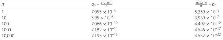
The following numerical computations (see Table1) would show that, forn∈N, Eq. (3.6) is sharper than Eq. (3.5).

In fact, we have, asn→ ∞,

arctann

n =an+O

1

n4

and arctann

n =bn+O

1

n5

.

4 Approximations toarctanx

For later use, we introduce the Padé approximant (see [13–16]). Letf be a formal power series,

f(t) =c0+c1t+c2t2+· · ·. (4.1)

The Padé approximation of order (p,q) of the functionf is the rational function, denoted by

[p/q]f(t) =

p j=0ajtj 1 +q_j=1bjtj

, (4.2)

Table 1 Comparison between approximation formulas (3.5) and (3.6).

n an–arctann n

arctann

n –bn

1 7.055×10–3 _5.259×10–3

10 5.95×10–6 _3.939×10–7

100 7.066×10–10 _4.492×10–12

1000 7.182×10–14 _4.546×10–17

wherep≥0 andq≥1 are two given integers, the coefficientsajandbjare given by (see [13–15])

⎧ ⎪ ⎪ ⎪ ⎪ ⎪ ⎪ ⎪ ⎪ ⎪ ⎪ ⎪ ⎪ ⎪ ⎪ ⎪ ⎪ ⎪ ⎪ ⎨ ⎪ ⎪ ⎪ ⎪ ⎪ ⎪ ⎪ ⎪ ⎪ ⎪ ⎪ ⎪ ⎪ ⎪ ⎪ ⎪ ⎪ ⎪ ⎩

a0=c0,

a1=c0b1+c1,

a2=c0b2+c1b1+c2, ..

.

ap=c0bp+· · ·+cp–1b1+cp,

0 =cp+1+cpb1+· · ·+cp–q+1bq, ..

.

0 =cp+q+cp+q–1b1+· · ·+cpbq,

(4.3)

and the following holds:

[p/q]f(t) –f(t) =O

tp+q+1. (4.4)

Thus, the firstp+q+ 1 coefficients of the series expansion of [p/q]f are identical to those off.

From the expansion (see [17, p. 81])

arctanx=π 2 +

∞

j=1

(–1)j

(2j– 1)x2j–1, |x|> 1,

we obtain

x

π

2 –arctanx

=

∞

j=0 cj

x2j= 1 – 1 3x2 +

1 5x4 –

1

7x6+· · ·, (4.5)

where

cj= (–1)j

2j+ 1 forj≥0. (4.6)

Let

f(t) =

∞

j=0 cj

tj, (4.7)

with the coefficientscjgiven in (4.6). Then we have

fx2=

∞

j=0 cj

x2j =x

π

2 –arctanx

. (4.8)

Based on the Padé approximation method, we now give a derivation of Eq. (1.10). To this end, we consider

[1/1]f(t) =

1 j=0ajt–j 1 +1_j=1bjt–j

.

Noting that

c0= 1, c1= – 1

3, c2= 1

5, (4.9)

holds, we have, by (4.3),

⎧ ⎪ ⎪ ⎨ ⎪ ⎪ ⎩

a0= 1,

a1=b1–1₃,

0 =1 5–

1 3b1,

that is,

a0= 1, a1= 4

15, b1= 3 5.

We thus obtain

[1/1]f(t) = 1 +₁₅4_t

1 +₅3_t =

15t+ 4

3(5t+ 3), (4.10)

and we have, by (4.4),

f(t) = 15t+ 4 3(5t+ 3)+O

1

t3

, t→ ∞. (4.11)

Replacingtbyx2in (4.11) yields (1.10).

From the Padé approximation method and the expansion (4.7), we now present a general result.

Theorem 4.1 The Padé approximation of order(p,q)of the function f(t) =∞_j=0c_tjj (at the point t=∞)is the following rational function:

[p/q]f(t) =

1 +p_j=1ajt–j

1 +q_j=1bjt–j

=tq–p

tp_+a

1tp–1+· · ·+ap

tq_+b

1tq–1+· · ·+bq

where p≥1and q≥1are any given integers,the coefficients ajand bjare given by

⎧ ⎪ ⎪ ⎪ ⎪ ⎪ ⎪ ⎪ ⎪ ⎪ ⎪ ⎪ ⎪ ⎪ ⎪ ⎪ ⎨ ⎪ ⎪ ⎪ ⎪ ⎪ ⎪ ⎪ ⎪ ⎪ ⎪ ⎪ ⎪ ⎪ ⎪ ⎪ ⎩

a1=b1+c1,

a2=b2+c1b1+c2, ..

.

ap=bp+· · ·+cp–1b1+cp,

0 =cp+1+cpb1+· · ·+cp–q+1bq, ..

.

0 =cp+q+cp+q–1b1+· · ·+cpbq,

(4.13)

and cjis given in(4.6),and the following holds:

f(t) – [p/q]f(t) =O

1

tp+q+1

, t→ ∞. (4.14)

In particular,replacing t by x2_{in(4.14)yields}

x

π

2 –arctanx

=x2(q–p)

x2p+a1x2(p–1)+· · ·+ap

x2q_+b

1x2(q–1)+· · ·+bq

+O

1

x2(p+q+1)

, x→ ∞, (4.15)

with the coefficients ajand bjgiven by(4.13).

Setting (p,q) = (k,k) in (4.15), we obtain the following corollary.

Corollary 4.1 As x→ ∞,

x

π

2 –arctanx

=x 2k_+a

1x2(k–1)+· · ·+ak

x2k_+b

1x2(k–1)+· · ·+bk +O

1

x4k+2

, (4.16)

where k≥1is any given integer,the coefficients ajand bj(1≤j≤k)are given by

⎧ ⎪ ⎪ ⎪ ⎪ ⎪ ⎪ ⎪ ⎪ ⎪ ⎪ ⎪ ⎪ ⎪ ⎪ ⎪ ⎨ ⎪ ⎪ ⎪ ⎪ ⎪ ⎪ ⎪ ⎪ ⎪ ⎪ ⎪ ⎪ ⎪ ⎪ ⎪ ⎩

a1=b1+c1,

a2=b2+c1b1+c2, ..

.

ak=bk+· · ·+ck–1b1+ck,

0 =ck+1+ckb1+· · ·+c1bk, ..

.

0 =c2k+c2k–1b1+· · ·+ckbk,

(4.17)

Settingk= 2 in (4.16) yields, asx→ ∞,

x

π

2 –arctanx

= 945x

4_{+ 735x}2_{+ 64}

15(63x4_{+ 70x}2_{+ 15)}+O

1

x10

, (4.18)

which gives

arctanx=π 2 –

945x4_{+ 735x}2_{+ 64} 15x(63x4_{+ 70x}2_{+ 15)}+O

1

x11

.

Using the Maple software, we find, asx→ ∞,

arctanx=π 2 –

945x4+ 735x2+ 64 15x(63x4_{+ 70x}2_{+ 15)}+

64 43,659x11

– 1856 464,373x13+O

1

x15

. (4.19)

Equation (4.19) motivated us to establish new bounds forarctanx.

Theorem 4.2 For x> 0,we have

π

2 –

945x4_{+ 735x}2_{+ 64} 15x(63x4_{+ 70x}2_{+ 15)}+

64 43,659x11–

1856 464,373x13

<arctanx<π 2 –

945x4_{+ 735x}2_{+ 64} 15x(63x4_{+ 70x}2_{+ 15)}+

64

43,659x11. (4.20)

Proof Forx> 0, let

I(x) =arctanx–

π

2 –

945x4+ 735x2+ 64 15x(63x4_{+ 70x}2_{+ 15)}+

64 43,659x11 –

1856 464,373x13

and

J(x) =arctanx–

π

2 –

945x4_{+ 735x}2_{+ 64} 15x(63x4_{+ 70x}2_{+ 15)}+

64 43,659x11

.

Differentiation yields

I(x) = –64(230,391x

8_{+ 372,680x}6_{+ 236,885x}4_{+ 65,400x}2_{+ 6525)}

35,721x14_{(1 +x}2_)(63x4_{+ 70x}2_{+ 15)}2 < 0

and

J(x) = 64(12,789x

8_{+ 15,610x}6_{+ 8890x}4_{+ 2325x}2_{+ 225)}

3969x12_{(1 +x}2_)(63x4_{+ 70x}2_{+ 15)}2 > 0.

Hence,I(x) is strictly decreasing andJ(x) is strictly increasing forx> 0, and we have

I(x) > lim

t→∞I(t) = 0 and J(x) <tlim→∞J(t) = 0 forx> 0.

Remark4.1 We point out that, forx> 1.0213 . . . , the lower bound in (4.20) is better than the one in (1.7). Forx> 0.854439 . . . , the upper bound in (4.20) is better than the one in (1.7). Forx> 0.947273 . . . , the lower bound in (4.20) is better than the one in (3.1). For

x> 0.792793 . . . , the upper bound in (4.20) is better than the one in (3.1).

5 Conclusions

In this paper, we establish a symmetric double inequality forarctanx(Theorem3.1). We determine the coefficientsajandbj(1≤j≤k) such that

x

π

2 –arctanx

=x 2k_+a

1x2(k–1)+· · ·+ak

x2k_+b

1x2(k–1)+· · ·+bk +O

1

x4k+2

, x→ ∞,

where k≥1 is any given integer (see Corollary4.1). Based on the obtained result, we establish new bounds forarctanx(Theorem4.2).

Appendix: A derivation of (1.8), (1.9), and (1.10)

Define the functionF(x) by

F(x) =arctanx

x –

1

a+√b+cx2.

We are interested in finding the values of the parametersa,b, andcsuch thatF(x) con-verges as fast as possible to zero, asx→ ∞. This provides the best approximations of the form

arctanx

x ≈

1

a+√b+cx2, x→ ∞.

Using the Maple software, we find, asx→ ∞,

F(x) =π √

c– 2 2√cx +

a–c cx2 +

b– 2a2

2c3/2_x3

+3a

3_+c2_{– 3ab}

3c2_x4 +O

1

x5

.

The three parametersa,b, andc, which produce the fastest convergence of the function

F(x), are given by

⎧ ⎪ ⎪ ⎨ ⎪ ⎪ ⎩

π√c– 2 = 0,

a–c= 0,

b– 2a2_{= 0,}

namely, if

a= 4

π2, b= 32

π4, c= 4

We then obtain, asx→ ∞,

arctanx

x =

1

4 π2 +

32 π4+_π42x2

–12 –π 2

3π2_x4 +O

1

x5

= π

2

4 +32 + (2πx)2 – 12 –π2

3π2_x4 +O

1

x5

.

Define the functionG(x) by

G(x) =arctanx

x –

1

p+q+rx+sx2.

Using the Maple software, we find, asx→ ∞,

G(x) =π √

s– 2 2√sx +

r– 2s3/2_{+ 2p}√_s 2s3/2_x2 +

4qs– 3r2_{– 8sp}2_{– 8}√_spr 8s5/2_x3

+–48s

3/2_{pq+ 48}√_spr2_{– 36rqs+ 15r}3_{+ 48s}3/2_p3_{+ 72sp}2_{r+ 16s}7/2

48s7/2_x4

+120sqr2– 128√spr3– 128s2p4– 240sp2r2+ 256rs3/2pq+ 192s2p2q

– 256s3/2p3r– 35r4– 48q2s2/128s9/2x5

+O

1

x6

.

For

p=24 –π 2

3π2 , q=

432 – 24π2_+π4

9π4 , r= –

4(12 –π2₎

3π3 , s= 4

π2,

we obtain, asx→ ∞,

arctanx

x =

3π2

24 –π2_{+432 – 24π}2_+π4_{– 12π(12 –π}2_{)x+ (6πx)}2

+π 4_{– 72}

18π3_x5 +O

1

x6

.

Define the functionH(x) by

H(x) =x

π

2 –arctanx

–x 2_+a

1x+a2 x2_+b

1x+b2 .

Using the Maple software, we find, asx→ ∞,

H(x) =b1–a1

x –

3a2– 3b2– 3a1b1+ 3b21+ 1

3x2 +

a1b2– 2b1b2+a2b1–a1b21+b31 x3

––1 – 5a2b2+ 5b 2

2+ 10a1b1b2– 15b21b2+ 5a2b21– 5a1b31+ 5b41 5x4

+–a1b 2

2+ 3b1b22– 2a2b1b2+ 3a1b21b2– 4b31b2+a2b13–a1b41+b51

x5 +O

1

x6

For

a1= 0, b1= 0, a2= 4

15, b2= 3 5,

we obtain, asx→ ∞,

x

π

2 –arctanx

=x 2₊ 4

15 x2₊3 5

+O

1

x6

.

Acknowledgements

We thank the editor and referees for their careful reading and valuable suggestions to make the article more easily readable.

Funding Not applicable.

Competing interests

The authors declare that they have no competing interests.

Authors’ contributions

Both authors contributed equally to this work. Both authors read and approved the final manuscript.

Publisher’s Note

Springer Nature remains neutral with regard to jurisdictional claims in published maps and institutional affiliations.

Received: 26 January 2018 Accepted: 13 June 2018 References

1. Shafer, R.E.: Problem E1867. Am. Math. Mon.73, 309 (1966)

2. Shafer, R.E.: Problems E1867 (solution). Am. Math. Mon.74, 726–727 (1967)

3. Qi, F., Zhang, S.Q., Guo, B.N.: Sharpening and generalizations of Shafer’s inequality for the arc tangent function. J. Inequal. Appl.2009, Article ID 930294 (2009).https://doi.org/10.1155/2009/930294

4. Qi, F., Niu, D.W., Guo, B.N.: Refinements, generalizations, and applications of Jordan’s inequality and related problems. J. Inequal. Appl.2009, Article ID 271923 (2009).https://doi.org/10.1155/2009/271923

5. Chen, X.D., Shi, J., Wang, Y., Pan, X.: A new method for sharpening the bounds of several special functions. Results Math.72, 695–702 (2017).https://doi.org/10.1007/s00025-017-0700-x

6. Chen, C.P., Cheung, W.S., Wang, W.: On Shafer and Carlson inequalities. J. Inequal. Appl.2011, Article ID 840206 (2011). https://doi.org/10.1155/2011/840206

7. Shafer, R.E.: On quadratic approximation. SIAM J. Numer. Anal.11, 447–460 (1974).https://doi.org/10.1137/0711037 8. Shafer, R.E.: Analytic inequalities obtained by quadratic approximation. Publ. Elektroteh. Fak. Univ. Beogr., Ser. Mat. Fiz.

57(598), 96–97 (1977)

9. Shafer, R.E.: On quadratic approximation, II. Publ. Elektroteh. Fak. Univ. Beogr., Ser. Mat. Fiz.602(633), 163–170 (1978) 10. Zhu, L.: On a quadratic estimate of Shafer. J. Math. Inequal.2, 571–574 (2008).

http://files.ele-math.com/articles/jmi-02-51.pdf

11. Sun, J.-L., Chen, C.-P.: Shafer-type inequalities for inverse trigonometric functions and Gauss lemniscate functions. J. Inequal. Appl.2016, 212 (2016).https://doi.org/10.1186/s13660-016-1157-2

12. Nishizawa, Y.: Refined quadratic estimations of Shafer’s inequality. J. Inequal. Appl.2017, 40 (2017). https://doi.org/10.1186/s13660-017-1312-4

13. Bercu, G.: Padé approximant related to remarkable inequalities involving trigonometric functions. J. Inequal. Appl. 2016, 99 (2016).https://doi.org/10.1186/s13660-016-1044-x

14. Bercu, G.: The natural approach of trigonometric inequalities—Padé approximant. J. Math. Inequal.11, 181–191 (2017).https://doi.org/10.7153/jmi-11-18

15. Bercu, G., Wu, S.: Refinements of certain hyperbolic inequalities via the Padé approximation method. J. Nonlinear Sci. Appl.9, 5011–5020 (2016).https://doi.org/10.22436/jnsa.009.07.05

16. Brezinski, C., Redivo-Zaglia, M.: New representations of Padé, Padé-type, and partial Padé approximants. J. Comput. Appl. Math.284, 69–77 (2015).https://doi.org/10.1016/j.cam.2014.07.007