http://dx.doi.org/10.4236/jamp.2015.32036
Quiet Zone Design in Diffuse Fields Using
Ultrasonic Transducers
Wen-Kung Tseng
Graduate Institute of Vehicle Engineering, National Changhua University of Education, Changhua City, Taiwan Email: [email protected]
Received 25 November 2014
Abstract
This paper presents quiet zone design using ultrasonic transducers for local active control in pure tone diffuse fields. Most of researches in local active noise control used conventional loudspeakers for the secondary sources to produce quiet zones. Recently ultrasonic transducers have been used for the secondary sources to control the plane wave in active noise control. However there is no research related to active noise control in diffuse fields using ultrasonic transducers. Therefore this study uses ultrasonic transducers for the secondary sources to control the diffuse fields. The quiet zone produced using ultrasonic transducers in single tone diffuse fields has been analyzed through simulations in this work. The results showed that quiet zones created using ultrasonic transducers were larger than those created using conventional loudspeakers. This is due to the fact that the audible sound pressure produced by the ultrasonic transducers decays slowly with the distance. Therefore the secondary field created by an ultrasonic transducer could fit the pri-mary field better and the larger zone of quiet could be obtained using the ultrasonic transducer. Also the audible sound produced by the ultrasonic transducers is directional; therefore the sound pressure amplification outside the quiet zones was lower.
Keywords
Quiet Zone Design, Ultrasonic Transducers, Local Active Control, Diffuse Fields, Plane Wave
1. Introduction
eliminate the possibility of sound coupling. It is foreseen that ultrasonic transducers enable ANC system to be more efficient [6] [7]. Despite the promising characteristics of ultrasonic transducers, it entails some side effect as well. Because of the strong directivity of sound, the target point is just limited along the radiation direction. If the target point shifts away from the radiation axis, ultrasonic transducers cannot cover the target point anymore unless the ultrasonic transducers mechanically rotate the face to trace the target, whereas a normal sound source does not have to [8] [9]. Therefore this study uses ultrasonic transducers for the secondary sources to control the diffuse fields. The optimization method has been used to control the pure tone diffuse fields and the quiet zone produced using ultrasonic transducers has also been analyzed through simulations in this work.
2. Design of Quiet Zones in Diffuse Fields
In this section the formulations for the design of the quiet zones in diffuse fields using ultrasonic transducers are presented. The primary field used in the work is assumed to be diffuse and comprised of many propagating plane waves with random amplitudes and phases, arriving from uniformly distributed directions. In this study 72 such incident plane waves together with random amplitudes and phases are chosen to generate an approximation of a diffuse sound field in order to be consistent with that of a previous work [1] [2]. The diffuse sound field was therefore generated by adding together the contributions of 12 plane waves in the azimuthal directions (corres-
ponding to azimuthal angles 300
L L
ϕ = × , L=1, 2, 3,,12) for each of six vertical incident directions
(cor-responding to vertical angles 0
30
K K
θ = × for K =1, 2,3,, 6). The net pressure at the point
(
x0,y0)
on the x − y plane due to the superposition of these 72 plane waves can be expressed as follows [1] [2]:(
)
max max(
)
(
(
)
)
0 0 0 0
1 1
, sin exp sin cos sin sin
K L
p KL KL K K L K L
K L
p x y a jb θ jk x θ ϕ y θ ϕ
= =
=
∑ ∑
+ + (1)where aKL+ jbKL account for the amplitudes and phases of these incident plane waves, k is the acoustic wave number, θK is the angle between the direction of the plane wave propagation and the z-axis, and ϕL is the angle between the direction of the plane wave propagation projected on the x-y plane and the x-axis. Both the real and imaginary parts of the complex pressure are chosen from a random population with Gaussian distribu-tion N
( )
0,1 . Equation (1) was used to generate diffuse primary sound fields in the simulations presented below. The computation of the average diffuse field zone of quiet at a given frequency is based on an ensemble of 50 samples of diffuse fields calculated over a grid of 131 × 131 points in the x-y plane. The primary field samples are calculated once and then used in the calculation of the various controlled fields.The ultrasonic transducer is used as the secondary source in this study, since the directional audible sound field produced by the ultrasonic transducer does not decay rapidly as the distance is increased. Therefore larger quiet zones could be obtained using the ultrasonic transducer. The sound pressure at a field point
(
x y,)
of the secondary waves produced by the ultrasonic transducer was derive by Westervelt [8] and can be expressed as follows.( )
2
0 0
0
e e sin cos 2
,
s qr p vx q q
s s v s s v
l s
v q
r r
t k x m t k x
c c
p x y AS
r
α α ω ω
− −
=
− − − − −
=
∑
(2)where
2 2
0 4 0 0
4π s
P m
A
c
β ω ρ
= , S=δ δy z, l denotes the effective source length, p0 is the sound pressure amplitude,
β is the nonlinear factor, m is the modulation index, rq = r2+x2−2 cosrx θ , αs is the absorption coeffi- cient of the audible sound, αp is the absorption coefficient of the carrier wave, ρ0 is the air density, c0 is
the sound speed.
Therefore the total acoustic pressure at a field point
(
x y,)
due to both the diffuse primary field and the sin-gle secondary source can be expressed as(
,)
(
,)
(
,)
T p s
p x y = p x y +p x y (3)
( )
max max(
)
(
(
)
)
1 12
0 0
0
, sin exp sin cos sin sin
e e sin cos 2
.
s q p v
K L
T KL KL K K L K L
K L
r x q q
s s v s s v
l
v q
p x y a jb jk x y
r r
t k x m t k x
c c
AS
r
α α
θ θ ϕ θ ϕ
ω ω = = − − = = + + − − − − − +
∑ ∑
∑
(4)If two secondary sources are used the total acoustic pressure at a field point
(
x y,)
can be expressed as( )
max max(
)
(
(
)
)
1 1 1
2 1 1
0 0
1
0 1
, sin exp sin cos sin sin
e e sin cos 2
s q p v
K L
T KL KL K K L K L
K L
r x q q
s s v s s v
l
v q
p x y a jb jk x y
r r
t k x m t k x
c c
A S
r
α α
θ θ ϕ θ ϕ
ω ω = = − − = = + + − − − − − +
∑ ∑
∑
2 2 2 2
0 0
2
0 2
e e sin cos 2
.
s qr p vx q q
s s v s s v
l
v q
r r
t k x m t k x
c c
A S
r
α α ω ω
− − = − − − − − +
∑
(5) where 2 2 10 1 4 0 0 4π s P m A c β ω ρ= and
2 2 20 2 4 0 0 4π s P m A c β ω ρ
= . In this study an optimization method is used to control the pure
tone diffuse field. The cost function can be expressed as.
(
)
max max(
)
(
(
)
)
1 2
2
, , 1 1
2 1 1
0 0
1
, sin exp sin cos sin sin
e e sin cos 2
s q ij p vi
K L
T i j KL KL K i K L j K L i j i j K L
r x q ij q ij
s s vi s s vi
J P x y a jb jk x y
r r
t k x m t k x
c c
A S
α α
θ θ ϕ θ ϕ
ω ω = = − − = = + + − − − − − +
∑
∑ ∑ ∑
2 0 1 22 2 2
0 0
2
0 2
e e sin cos 2
.
s q ij p vi
l
v q ij
r x q ij q ij
s s vi s s vi l
v q ij
r
r r
t k x m t k x
c c
A S
r
α α ω ω
= − − = − − − − − +
∑
∑
(6)For the amplification limit, a constraint could be added to the optimization process as follows.
(
)
(
(
)
)
max max
1
2 1 1
2 1 1
0 0
1
0 1
2
2
20log sin exp sin cos sin sin
e e sin cos 2
e e
s q ij p vi
s q ij p
K L
KL KL K i K L j K L K L
r x q ij q ij
s s vi s s vi l
v q ij
r
a jb jk x y
r r
t k x m t k x
c c A S r A S α α α α
θ θ ϕ θ ϕ
ω ω = = − − = − − + + − − − − − + +
∑ ∑
∑
2 2 0 0 0 2sin cos 2
,
at somepoints outside the quiet zone.
vi
x q ij q ij
s s vi s s vi l
v q ij
r r
t k x m t k x
c c r ω ω σ = − − − − −
<
∑
where σ is the dB value of the amplification limit. Therefore the formulation of the optimization problem can be written as follows.
Minimize
(
)
(
(
)
)
max max
1
2
, 1 1
2 1 1
0 0
1
0 1
2
2
sin exp sin cos sin sin
e e sin cos 2
e e
s q ij p vi
s q ij p
K L
KL KL K i K L j K L
i j K L
r x q ij q ij
s s vi s s vi
l
v q ij
r x
a jb jk x y
r r
t k x m t k x
c c A S r A S α α α α
θ θ ϕ θ ϕ
ω ω = = − − = − − + + − − − − − + +
∑ ∑ ∑
∑
2 2 2 0 0 0 2sin cos 2
.
vi q ij q ij
s s vi s s vi
l
v q ij
r r
t k x m t k x
c c r ω ω = − − − − −
∑
Subject to(
)
(
(
)
)
max max 1 2 1 12 1 1
0 0
1
0 1
2
2
20log sin exp sin cos sin sin
e e sin cos 2
e e
s q ij p vi
s q ij p
K L
KL KL K i K L j K L
K L
r x q ij q ij
s s vi s s vi
l
v q ij
r
a jb jk x y
r r
t k x m t k x
c c A S r A S α α α α
θ θ ϕ θ ϕ
ω ω = = − − = − − + + − − − − − + +
∑ ∑
∑
2 2 0 0 0 2sin cos 2
,
at some points outside the quiet zone.
vi
x q ij q ij
s s vi s s vi
l
v q ij
r r
t k x m t k x
c c r ω ω σ = − − − − −
<
∑
(8)
The optimal values of A1 and A2 can be calculated using the function fmincon
( )
in MATLAB.Substi-tuting the optimal values of A1 and A2 into Equation (5), the controlled field, PT
(
x y,)
, can be calculated foreach diffuse field sample at each position
(
x y,)
in the quiet zone.3. Simulation Results
In this section the simulation results for average zones of quiet created by one, two and three secondary sources using ultrasonic transducers seeking to minimize the squared pressure in the minimization area in a pure tone diffuse primary field are presented. The quiet zones are also compared to those obtained by using the conven-tional loudspeakers. In the first simulation, the secondary fields created using a single ultrasonic transducer and a conventional loudspeaker are compared as shown in Figure 1. As can be seen from the figure the secondary field produced by an ultrasonic transducer decays slowly when the distance increases. However the secondary field produced by a conventional loudspeaker decays fast when the distance increases.
Figure 1. The secondary field: (-) an ultrasonic transducer, (_.) a conventional loudspeaker.
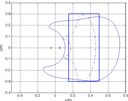
primary field for k=2 is generated in this case, where k is the acoustic wave number. This will correspond to an excitation frequency of 108 Hz. Figure 2 shows the 10 dB reduction contour line in the calculated average zone of quiet created using an ultrasonic transducer (solid line) inside a desired quiet zone area represented by the rectangular frame for 108 Hz. Also shown is the 10 dB reduction contour line created using a conventional loudspeaker (dash-dot line). The secondary source is marked as a star. It can be seen that the zone of quiet created using an ultrasonic transducer is larger than that created using a conventional loudspeaker over this carefully selected area. This is due to the fact that the secondary field produced by a single ultrasonic transducer decays slowly, resulting in some difference on the secondary field shape. Therefore the secondary field created by an ultrasonic transducer could fit the primary field better and the larger zone of quiet could be obtained using the ultrasonic transducer.
A single ultrasonic transducer can only produce a simple decaying field. If two ultrasonic transducers are used, more complicated secondary fields can be produced. Therefore larger zones of quiet could be expected to be ob-tained. In the next simulations two ultrasonic transducers are introduced to minimize the acoustic pressure in the minimization area. The zones of quiet are then compared to those designed by using two conventional louds-peakers. Figure 3 shows the 10 dB reduction contour line (solid line) in the calculated average zones of quiet for two ultrasonic transducers with the desired quiet zone represented by the bold rectangular frame for 108 Hz. Also shown is the 10 dB reduction contour line (dash-dot line) for two conventional loudspeakers with the mi-nimization area represented by the bold rectangular frame. The two secondary sources located at (0.05, 0) and (−0.05, 0) are marked by stars. Previous work showed that minimizing the acoustic pressure over an area by us-ing 2-norm minimization with conventional loudspeakers produced a larger zone enclosed by the 10dB reduc-tion contour compared to that created when cancelling the acoustic pressure and particle velocity at one point (Garcia-Bonito et al., 1997; Tseng et al., 2000). However Figure 3 shows that using two ultrasonic transducers produce a larger zone enclosed by the 10dB reduction contour compared to that created when using two conven-tional loudspeakers.
4. Conclusion
[image:5.595.178.418.83.275.2]Figure 2. The 10 dB reduction contour of the average zone of quiet created by a secondary source located at position (0, 0), minimizing the acoustic pressure at an area represented by a bold rectangular frame using a conven-tional loudspeaker (dash-dot line) and an ultrasonic transducer (solid line) for 108 Hz.
Figure 3. The 10 dB reduction contour of the average zone of quiet created
by two secondary sources located at positions (0.05, 0) and (−0.05, 0),
mini-mizing the acoustic pressure at an area represented by a bold rectangular frame using two conventional loudspeakers (dash-dot line) and two ultrasonic transducers (solid line) for 108 Hz.
Acknowledgements
The study was supported by the Ministry of Science and Technology of Taiwan, under project number MOST 103-2221-E-018-005-.
References
[1] Tseng, W.K., Rafaely, B. and Elliott, S.J. (2000) Local Active Sound Control Using 2-Norm and ∞-Norm Pressure
Minimization. Journal of Sound and Vibration, 234, 427-439. http://dx.doi.org/10.1006/jsvi.1999.2889
[2] Elliott, S.J. and Garcia-Bonito, J. (1995) Active Cancellation of Pressure and Pressure Gradient in a Diffuse Sound
Field. Journal of Sound and Vibration, 186, 696-704. http://dx.doi.org/10.1006/jsvi.1995.0482
[3] Tseng, W.-K., Rafaely, B. and Elliott, S.J. (2012) A Novel Method of Designing Stable Feedback Controllers for Local
[image:6.595.189.410.86.261.2] [image:6.595.188.410.334.509.2][4] Puttmer, A. (2006) New Applications for Ultrasonic Sensors in Process Industries. Journal of Ultrasonic, 44, 1379-
1383. http://dx.doi.org/10.1016/j.ultras.2006.05.047
[5] Tanaka, N. and Tanaka, M. (2010) Active Noise Control Using a Steerable Parametric Array Loudspeaker. Journal of
Acoustical Society of America, 127, 3526-3537. http://dx.doi.org/10.1121/1.3409483
[6] Ju, H.S. and Kim, Y.H. (2010) Near-Field Characteristics of the Parametric Loudspeaker Using Ultrasonic Transducers.
Journal of Applied Acoustics, 71, 793-800. http://dx.doi.org/10.1016/j.apacoust.2010.04.004
[7] Brooks, L.A. (2005) Investigation into the Feasibility of Using a Parametric Array Control Source in an Active Noise
Control System. Proceedings of the ACOUSTICS 2005, 39-45.
[8] Westervelt, P.J. (1963) Parametric Acoustic Array. J. Acoust. Soc. Am., 35, 535-537.
http://dx.doi.org/10.1121/1.1918525
[9] Tan, K.S., Gan, W.S., Yang, J. and Er, M.H. (2003) Constant Beamwidth Beamformer for Difference Frequency in
Parametric Array. Proceedings of the IEEE International Conference on Acoustics, Speech and Signal Processing ICASSP,