Design and CFD Analysis of The Intake Manifold for the Suzuki G13bb Engine

Design and CFD Analysis of The Intake Manifold

for the Suzuki G13bb Engine

Abhishek Chaubey1, Prof. A.C. Tiwari2

1_{M. Tech student,} 2_{Head of department, Department of Mechanical Engineering}

University Institute of Technology, Rajiv Gandhi Proudyogiki Vishwavidyalaya, Bhopal, Madhya Pradesh, India

Abstract: This paper deals with the improvement of the performance and to achieve the even distribution of flow at each cylinders, to select the best turbulence model for the analysis of intake manifold using computational fluid dynamics, to achieve the maximum mass flow rate through the runners, to maintain the equal pressure throughout the plenum, to propagate back the higher pressure column of air to intake port within the duration of the intake valve’s closure. To achieve the even flow of distribution and improve the volumetric efficiency, author divided his analysis into three different parts. In each part, a different iteration of inlet manifold used in Maruti Gypsy’s G13BB engine are used. In this analysis plenum size is kept constant to show the effects of shape of runners on output. Dividing the work into three different parts provide the greater refinement in result. Runner shape is determined by the operating conditions of the engine assembly in which the inlet manifold is used. The intake runner diameter influences the point at which peak power is reached while the intake runner length will influence the amount of power available at high and low RPM. To find the best results, author perform the experiments in Ansys Fluent for possible designs and find the effect of curved and helical shape runners were providing higher volumetric efficiency and even flow of distribution to each cylinder. For designing final intake manifold author select best design from all three parts and perform the experiment using computational fluid dynamics software Ansys Fluent.

Keywords

:

I. INTRODUCTION

The main purpose of the intake manifold is to evenly distribute the combustion mixture to each intake port of the engine cylinder, unless the engine has direct injection [1]. Even distribution is important to optimize the volumetric efficiency and performance of the engine. There are various factors that influence the engine performance such as compression ratio, atomization of fuel, fuel injection pressure, and quality of fuel, combustion rate, air fuel ratio, intake temperature and pressure and also based on piston design, inlet manifold, and combustion chamber designs etc.

Geometrical design of intake manifold is one such method for the better performance of an I.C. Engine. Air swirl motion in engine influences the atomization and distribution of fuel injected in the combustion chamber. Intake manifolds provides Air motion to the chamber.

Almost every researchers and automotive industry is focused on improvement of intake manifold. However, there is always room for enhancement on intake system. The air intake system has seen many reiterations and improvements and substantially increased during the past years by controlling the dimension and shape, and permitting the engine to produce increasing amounts of power by improving their volumetric efficiency, best possible fuel consumption, reduced fuel emissions, and most of the research performed, by automotive researchers and engine manufacturers (i.e. Mazda, BMW, Audi, Ford, Renault etc.) [2]. Porsche in the 1980s developed an intake system to use on their vehicles that adjusted the length of the intake system by switching amongst the longer and shorter pair of tube utilizing a butterfly valve, developing some positive pressure, which usually enhances overall performance of the engine. Audi began to use a similar system in some cars in the 1990s and Ford Motor in 1997 [3].

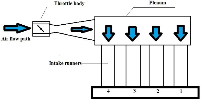
II. NOMENCLATURE OF INTAKE SYSTEM

Figure 1: Body of Intake Manifold

The information of the work which has been done formerly on intake manifolds allow a more systematic discussion of intake system. On the basis of those information and facts, the basic of acoustic wave theory and general terminology of intakes will be the major field of study, the general terminologies of intake system, which can be used for improvement are:

1) Plenum: It is storage device which placed between throttle valve and cylinder runner. The function of the plenum is to equalize pressure for more even distribution air-fuel mixture in side combustion chamber, because of irregular supply or demand of the engine cylinder, sometime plenum chamber also work as an acoustic silencer device. There are two types of intake manifold on the basis of manifold dimension, fixed length intake manifold and variable length intake manifold.

2) Cylinder Runner: The cylinder runners are the parts of the air intake system which delivers air from plenum to the combustion chamber. In each runner, the principal phenomenon that governs its performance is actually, the effect of acoustic waves. As the purpose of the cylinder runner is distribution of air, performance to transport the maximum amount of air, and in the case of the engine, the successive enhancement in volumetric efficiency.

III. BASICS OF COMPUTATIONAL FLUID DYNAMICS (CFD)

Computational Fluid Dynamics, known as CFD, is defined as the set of methodologies that enable the computer to provide us with a numerical simulation of fluid flows. We use the word ‘simulation’ to indicate that we use the computer to solve numerically the laws that govern the movement of fluids, in or around a material system, where its geometry is also modeled on the computer. Hence, the whole system is transformed into a ‘virtual’ environment or virtual product. This can be opposed to an experimental investigation, characterized by a material model or prototype of the system, such as an aircraft or car model in a wind tunnel, or when measuring the flow properties in a prototype of an engine. This terminology is also referring to the fact that we can visualize the whole system and its behavior, through computer visualization tools, with amazing levels of realism, as you certainly have experienced through the powerful computer games and/or movie animations, which provide a fascinating level of high-fidelity rendering. Hence the complete system, such as a car, an airplane, a block of buildings, etc. can be ‘seen’ on a computer, before any part is ever constructed.

A. Virtual prototyping in CFD

and Computer-Assisted Manufacturing (CAM) software. The CAD/CAE/CAM software systems form the basis for the different phases of the virtual prototyping environment. There are components of a computer-oriented environment, as used in industry to create, or modify toward better properties, of a product. This product can be a single component such as a cooling jacket in a car engine, formed by a certain number of circular curved pipes, down to a complete car. In all cases the succession of steps and the related software tools are used in very much similar ways, the difference being the degree of complexity to which these tools are applied.

IV. PHASES OF CREATION IN CFD

A. The Definition Phase

The first step in the creation of the product is the definition phase, which covers the specification and geometrical definition. It is based on CAD software, which allows creating and defining the geometry of the system, in all its details. Typically, large industries can employ up to thousands of designers, working full time on CAD software. Their day-to-day task is to build the geometrical model on the computer screen, in interaction with the engineers of the simulation and analysis departments.

This CAD definition of the geometry is the required and unavoidable input to the CFD simulation task. Its application cover a very wide range of applications, industrial, environmental and bio-medical. Environmental studies of wind effects around a block of buildings, with the main objective to improve the wind comfort of the people walking close to the main buildings. In CAD definition of an aircraft, CFD study helps to simulate the flow around it. Several branches of the lung and the CFD analysis has as objective to determine the airflow configuration during inspiration and to determine the path of inhaled aerosols, typical of medical sprays, in function of the size of the particles. It is of considerable importance for the medical and pharmaceutical sector to make sure that the inhaled medication will penetrate deep enough in the lungs as to provide the maximal healing effect. A CFD analysis is applied in both cases to improve the operating characteristics of these components and define appropriate geometrical changes.

B. The Simulation and Analysis Phase

The next phase is the simulation and analysis phase, which applies software tools to calculate, on the computer, the physical behavior of the system. This is called virtual prototyping. This phase is based on CAE software (eventually supported by experimental tests at a later stage), with several sub-branches related to the different physical effects that have to be modeled and simulated during the design process. The most important of these are:

1) Computational Solid Mechanics (CSM): The software tools able to evaluate the mechanical stresses, deformations, vibrations of the solid parts of a system, including fatigue and eventually life estimations. Generally, CSM software will also contain modules for the thermal analysis of materials, including heat conduction, thermal stresses and thermal dilation effects. Advanced software tools also exist for simulation of complex phenomena, such as crash, largely used in the automotive sector and allowing considerable savings, when compared with the cost of real crash experiments of cars being driven into walls 2) Computational Fluid Dynamics (CFD): It is designated as the software tools that allow the analysis of the fluid flow, including

the thermal heat transfer and heat conduction effects in the fluid and through the solid boundaries of the flow domain. For instance, in the case of an aircraft engine, CFD software will be used to analyze the flow in the multistage combination of rotating and fixed blade rows of the compressor and turbine; predict their performance; analyze the combustor behavior, analyze the thermal parts to optimize the cooling passages, cavities, labyrinths, seals and similar sub-components. A growing number of sub-components are currently being investigated with CFD tools; while the ultimate objective is to be able to simulate the complete engine, from compressor entry to nozzle exit.

3) Other simulation areas related to specialized physical phenomena are also currently applied and/or in development, such as Computational Aero-Acoustics (CAA) and Computational electromagnetics (CEM). They play an important role when effects such as reduction of noise or electromagnetic interferences and signatures are important design objectives.

V. PROBLEM DESCRIPTION

A. Selection Turbulence Model

The CFD analyses were conducted using the regular k-e turbulent model, and a first order upwind difference scheme. This model employs two additional transport equations one for turbulence kinetic energy (k) and another one for the dissipation rate (e).These solver settings guaranteed existence of a fully converged solution for each set of parameters. The optimization technique required high CFD accuracy for the evaluation of objective and constrain functions to compute the sensitivity for each variable. The CFD mesh was kept relatively coarse. Near wall treatment is handled through generalized wall functions. This model is well established and the most widely validated turbulence model.

B. Selection Of A Base Inlet Manifold

Inlet manifold used in G13BB engine manufactured by Suzuki Motor Corporation. The Single overhead camshaft (SOHC) 16-valve G13BB (introduced in March 1995) has electronic Multi-point fuel injection MPFI, generating 56–63 kW (76–86 PS) and 104–115 Nm (77–85 lb. ft). Later G13BBs have two coil packs bolted directly to the valve cover, although early models still had the coil packs mounted to the left side of the head, where the distributor was traditionally located. This engine is equipped with MAP sensor to monitor pressure in manifold, unlike the G16 series. This engine has a non-interference valve train design.

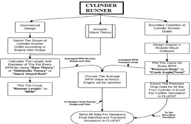
C. Selection Of Best Cylinder Runner Size And Boundary Condition

This stage deals with design methodology of cylinder runner and their boundary condition. In this stage author divided his work two part, first part was geometrical design methodology of cylinder runner by using Ram Theory or Helmholtz Theory

1) Ram theory: Air flowing inside the intake manifold runner, past the intake valve and into the cylinder flows alike until the intake valve closes. After the closure of valve air strikes on the closed valve & high pressure wave is created. This high pressure wave oscillates in the inlet duct until the inlet valve opens for next stroke. The time after which inlet valve opens again if matches to the time of arrival of high pressure wave of air at inlet then Ram effect occurs causing highest possible air pressure at IVC. Tuning corresponds to adjusting the length of intake runner so that this pressure wave reaches exactly at the time when the inlet valve opens. This effect is also called as inertial ram effect and length is decided by Ram Theory.

2) Helmholtz Resonator Theory : This considers the volume of air inside the intake runner as spring which compresses & expands upon application of force to it. The air inside combustion chamber is considered as mass. Effective volume is considered to be the cylinder volume at the mid stroke. Following figure shows the arrangement.

Figure 2:Designing techniques for intake manifold for computer simulation

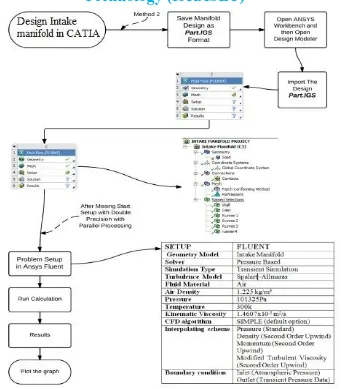
D. Simulation Setup Method

Figure 3: Simulation setup in Ansys Fluent

The flow pattern in the intake region is insensitive to flow unsteadiness and valve operation and thus could be predicted through steady flow test and computational simulation with reasonable accuracy.

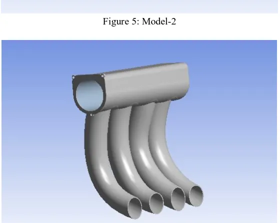
A new manifold needs to be designed to improve the performance of the engine. Two such configurations have been made as shown the figures 5 and 6. The first manifold is the original manifold. Second and third manifolds are made such that the curvature of runners in the second manifold provides both curved and helical runners branching together to provide for both low and high speed operation and in the third manifold radius of curvature of original inlet manifold is increased to provide a unrestricted air flow for high load engine operations. This gives the opportunity to observe the flow motion in each of the cases. The fillets on the manifold are chosen randomly. Internal volume solid or inverse volume of these of these manifolds are shown in figure 7. The first manifold is designated “model 1”, second manifold as “model 2”and the third manifold as “model 3”.

VI. RESULTS

A. CFD Simulation result

Figure 4: Model-1 (Actual Flow Model)

Figure 5: Model-2 (Model with branched helical runners) Figure 6: Model-3 (Model without curve of runner part)

Figure 4:Model-1

Figure 5: Model-2

For CFD simulation the internal volume of these models are generated by Boolean expressions in CATIATM _{also known as inverse}

volume of the design.

Figure 7:Inverse volumes of model 1, 2, 3

B. Dimensions of IM model

Table 1: Dimensions of intake manifold models (in mm)

Parameters Model 1 Model 2 Model 3

Radius 26.15 28.05 26.15

Length of plenum 233.6 264.5 233.6

Radius of runner 18.1 25.078 31.9

(a)

(a)Streamlines for FO: 1-3 for the model-1

(b) Streamlines for FO: 2-4 for the model-1 Figure 9: (a) & (b)

Table 2: Intake Port Configurations

Configurations Outlet 1 Outlet 2 Outlet 3 Outlet 4

FO: 1-3 Open Close Open Close

FO: 2-4 close Open Close Open

These configurations were investigated for each engine operating conditions by varying inlet velocities and outlet velocities were determined in CFD post. In CFD post, contours were created at inlet and outlet ports of the respective IM. Then using solution viewer, color pattern at the outlets was converted to numerical values of the outlet velocities in (m/s). Coordinates of the port was determined in the software itself. Inlet velocities at the inlet where outlet parameters are calculated are: 5m/s, 8.4 m/s, 11.2 m/s, 12.5m/s, 14m/s. For uniform charge distribution in all the runners the outlet is considered to be all the four runners since due to high speed the discharge would behave like it is occurring from all the four runners in same instant.

C. Model-1 flow simulation

Figure 10:Streamlines inside the model-1

1) Results of model-1

Table 3:

Outlet 1 Outlet 2 Outlet 3 Outlet4

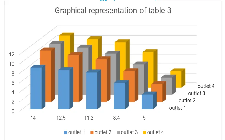
14 8.811 10.93 10.83 11.05

12.5 8.31 9.9499 9.9934 10.2307

11.2 7.79 9.05 8.75 9.6114

8.4 5.57 6.55 6.4194 7.5

Graph 1Velocities at the outlet of model 1

D. Model-2 flow simulation

Figure 11:Velocity contours at boundary in the model-2

Figure 12:Streamlines inside model-2

outlet 1 outlet 2

outlet 3 outlet 4

0 2 4 6 8 10 12

14 12.5 11.2 8.4 5

Graphical representation of table 3

1) Results of model-2

Table 4:

Outlet 1 Outlet 2 Outlet 3 Outlet 4

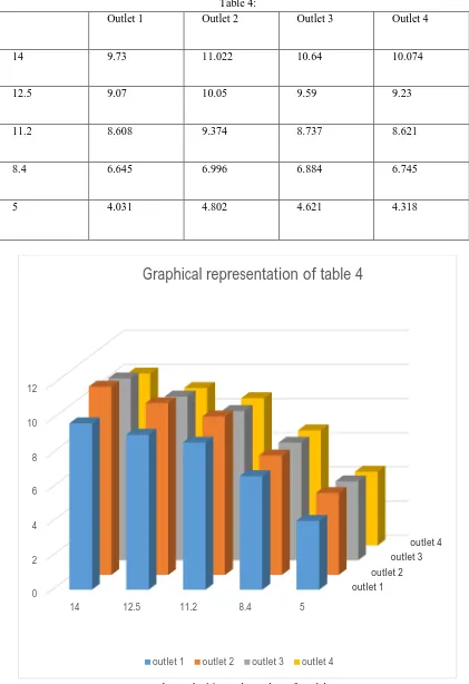
14 9.73 11.022 10.64 10.074

12.5 9.07 10.05 9.59 9.23

11.2 8.608 9.374 8.737 8.621

8.4 6.645 6.996 6.884 6.745

5 4.031 4.802 4.621 4.318

Graph 2 Velocities at the outlets of model 2

outlet 1 outlet 2

outlet 3 outlet 4

0 2 4 6 8 10 12

14 12.5 11.2 8.4 5

Graphical representation of table 4

E. Model-3 flow simulation

Figure 13: Streamlines inside the model-3 1) Results of model-3:

Table 5:

Outlet 1 Outlet 2 Outlet 3 Outlet 4

14 10.47 11.7486 11.0876 11.8862

12.5 9.323 10.71 10.35 10.53

11.2 8.295 9.6714 9.49 10.02

8.4 5.843 7.536 7.194 7.5458

Graph 3 Velocity at outlets of model 3

F. Examine the three models at different outlets:

Graph 4:Outlet vs. inlet velocities at outlet-1 of all 3 Models outlet 1

outlet 2 outlet 3

outlet 4

0 2 4 6 8 10 12

14 12.5 11.2 8.4 5

Graphical representation of table 5

outlet 1 outlet 2 outlet 3 outlet 4

0 2 4 6 8 10 12

14 12.5 11.2 8.4 5

Output 1

Graph 5:Outlet vs. inlet velocities at outlet-2 of all 3 Models

Graph 6:Outlet vs. inlet velocities at outlet-3 of all 3 Models

0 2 4 6 8 10 12

12.5 11.2 8.4 5

Output 2

Model 1 Model 2 Model 3

0 2 4 6 8 10 12

12.5 11.2 8.4 5

Output 3

Graph 7:Outlet vs. inlet velocities at outlet-4 of all 3 Models

1) Outlet 1: Model-1 shows lowest velocity among three models and lowest velocity among four runner also, it shows high radius of curvature in runner geometry has actual bad design configuration for high load vehicles.

2) Outlet 2 and Outlet 3: Graph shows difference in outlet velocity in Model-1 (actual model) and Model-3(model without curve) while the Model-2(model only with branched runners) show slight high value because of good design of curves at end of runners.

3) Outlet 4: At outlet 4 model-3 shows highest velocity among two models, the results at outlet 4 shows that may be the inside path of the flow inside the runner plays a significant role and helps in improving results of intake manifold

From the above charts we noticed that the model is good at the curving parts of runners and it helps in simulating the velocity equally at the four outlets.

G. Examine the three models at different inlet velocities:

Graph 8: Velocity at outlets vs. outlets of 3 models at Inlet velocity 14m/s

0 2 4 6 8 10 12

12.5 11.2 8.4 5

Output 4

Model 1 Model 2 Model 3

Model 1 Model 2 Model 3 0 2 4 6 8 10 12

1 2 3 4

Inlet velocity 14 m/s

Graph 9:Velocity at outlets vs. outlets of 3 model at Inlet velocity 12.5 m/s

Graph 10:Velocity at outlets vs. outlets of 3 models at Inlet velocity 11.2 m/s Model 1

Model 2 Model 3

0 2 4 6 8 10 12

1 2 3 4

Inlet velocity 12.5 m/s

Model 1 Model 2 Model 3

Model 1 Model 2

Model 3

0 2 4 6 8 10 12

1 2 3 4

Inlet velocity 11.2 m/s

Graph 11: Velocity at outlets vs. outlets of 3 models at Inlet velocity 8.4 m/s

Graph 12:Velocity at outlets vs. outlets of 3 models at Inlet velocity 5 m/s Model 1

Model 2 Model 3

0 1 2 3 4 5 6 7 8

1 2 3 4

Inlet velocity 8.4 m/s

Model 1 Model 2 Model 3

Model 1 Model 2

Model 3

0 1 2 3 4 5

1 2 3 4

Inlet velocity 5 m/s

Table 6: Percentage change in outlet velocity in model 2 with respect to model 1

Outlet 1 Outlet 2 Outlet 3 Outlet 4

14 10.430 0.840 -1.750 - 8.830

12.5 9.150 1.006 -4.036 -9.781

11.2 10.500 3.580 -0.148 -10.304

8.4 19.299 6.809 7.237 -10.066

5 30.0322 23.782 26.602 24.080

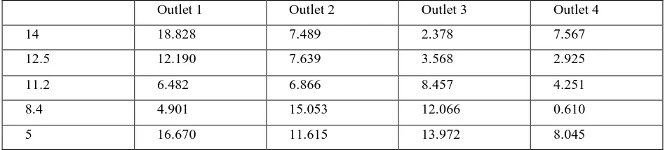
Table 7: Percentage change in outlet velocity in model 3 with respect to model 1

Outlet 1 Outlet 2 Outlet 3 Outlet 4

14 18.828 7.489 2.378 7.567

12.5 12.190 7.639 3.568 2.925

11.2 6.482 6.866 8.457 4.251

8.4 4.901 15.053 12.066 0.610

5 16.670 11.615 13.972 8.045

Maximum percentage change in outlet velocity in model 2 with respect to model 1= 30.0322 at 5m/s and outlet 1. Maximum percentage change in outlet velocity in model 3 with respect to model 1= 18.828 at 14m/s and outlet 1.

VII. CONCLUSION

After reviewing work of different authors as above it can be easily concluded that intake geometry made a considerable impact on outlet velocity. The main impact is on the volumetric efficiency of the engine which ultimately affects the torque & power produced at different engine speed. The intake manifold model 2 provides a straight and helical path for sir to flow and due to combination of these two outlets there is a high percentage increase of outlet velocity in model 2. Intake manifold model 3 is designed with less curvature at the runners. This is shown in results as there is a percentage increase in outlet velocity as compared to actual model. These 3 iterations of intake manifold for G13BB engine have to be selected accordingly in engines operating speed range. Longer intake manifolds give higher torque at lower RPMs while shorter intake manifold tends to give peak torque at high engine RPM. Author’s intention is towards studying the effect of shape of inlet manifold runners on outlet velocity and volumetric efficiency of the engine by theoretical & simulation methodologies.

Design software CATIATM _{served as a platform to obtain the configuration of the manifolds with different runner curvature and}

same plenum dimensions, while the CFD simulations enabled to visualize the flow within the manifold. Such simulations give better insight of flow within the manifolds. Design modifications could be done using CFD simulations to enhance the overall performance of the system. Using this method, a better design of manifold giving volumetric efficiency could be achieved.

VIII. ACKNOWLEDGEMENT

I would like to express my deep sense of gratitude and respect to my mentor Prof. Dr. A.C Tiwari, for his excellent guidance and suggestions. I express my gratitude towards our coordinator Dr. Rakesh Singhai for his insightful comments and contributions. I thank him for his kind help in preparation and presentation of this work.

REFERENCES

[1] Burtnett e. R. (1927). Inlet manifold for internal combustion engines. Available: www.google.com/patents/us1632880 [2] Sullivan d.a. (1939). Intake manifold. Available: www.google.com/patents/us2160922.

[3] Lee c.l. (1997). Variable air intake manifold. Available: www.google.com/patents/us5638785.

[4] Ceviz m.a and akin m., “design of a new si engine intake manifold with variable length plenum”, (2010).

[5] Safari m, nasiritosi a and ghamari m, “intake manifold optimization by using 3d- cfd analysis” sae paper, pp. 32-73, (2003). [6] Angner trindade. “use of 1d-3d coupled simulation to develop a intake manifold system” sae paper 01-1534, (2010). [7] Marcelo. R. C an

“intake manifold optimization by using 3-d cfd analysis” sae paper 32-0073, (2003)