uct
Software Effort Estimation using Satin Bowerbird
Algorithm
Rishi Kishore1, D. L. Gupta2
1
M.Tech student , 2Asso. Prof., Dept. of Computer Science and Engineering Kamla Nehru Institute of Technology, Sultanpur (UP) India
Abstract: There are various non-linear optimization problems can be effectively solved by Meta-heuristic Algorithms. The Software effort estimation is an optimization problem so it can also be solved by the Meta-heuristic algorithm. There are more than one algorithm is available today for finding the optimized solution for the particular problem. So we used one of the
Meta-heuristic algorithm that is Satin Bowerbird Algorithm[4]. This algorithm is used for finding the optimized value of a and b which
are used in the Boehm’s COCOMO[2][8] Model for finding the nearest result in terms of software effort estimation with the actual
effort as given in the dataset. We also used 15 effort multiplier for finding the nearest result. In recent years, the researchers try to pay more attention on the software effort estimation. In this paper we collate the software effort estimation among three
models, these are COCOMO Model[2][8], Genetic Algorithm and Satin Bowerbird Optimization Algorithm[4]. We also evaluate the
Mean Magnitude Relative Error and Root Mean Square value at last and compare with these models.
Keywords: COCOMO[2], Satin Bowerbird Optimization Algorithm, Genetic Algorithm[7][9]
I. INTRODUCTION
When we talk about the development of a software product then two things comes in our mind, first is the cost of the software product and second, the time taken by the software company to develop the software product. But when we talk about software development effort estimation that is the manpower to develop the software, two things are more important. One is the software development organization must develop models that are practically relevant and another is that, the organization considers the objective of effort estimation as a prime factor for accurately estimate a model. Software Effort estimation means the effort made by the software developers or programmer to develop the software product and it computes in terms of PM (Person-Month). Similarly the cost estimation is the total cost or budget of the software product, it contains all the cost from analyze to the publish of the software. Effort estimation is a process in which one can predict the development time and cost for developing a software process or a product. Estimated cost and accurate time to complete the project plays a vital role in software effort estimation. Because when the estimated cost is over then harm in financial loss will be there and when estimated cost is less than the actual then the organization may result in poor quality of software which eventually leads to failure of the software. Very less information is available at early stage but yet it is a challenging task for software engineers to evaluate effort estimation with that information only. Also Effort estimations done at an initial phases of development of a project may turn out to be helpful for project managers. There are many algorithmic and non-algorithmic methods available for effort estimation.
This review paper is organized as follows: in Section 2, we describe the literature review in which the software cost estimation in different models and algorithms are shown. In Section 3, the proposed model and evaluated result of the effort estimation using this model is shown. In Section 4, compare the estimated effort with table and graphs. And in Section 5, we present the conclusion and future work.
II. LITERATUREREVIEW
In this section, we present the existing models with brief introduction which are using for evaluating the software effort. These models are the Genetic Algorithm and the COCOMO model.
A. The Genetic Algorithm
better than the old one. Solutions which are selected from the population to form new solutions (called offspring) are selected pursuance to their fitness - the more suitable they have more chances to reproduce. This is repeated until some valid condition (improvement of the best solution) is satisfied.
Some of the terms used in the GA are familiar, so their explanations are given as follows.
1) Search Space: The space of all appropriate solutions (it means objects among those the desired solution) is known as search space (also called state space). Each solution in the search space represents one appropriate solution. Each appropriate solution can be "marked" as its value or fitness for the problem. We are looking for one appropriate solution among more solutions which are available in the search.
2) Pseudo Code for Genetic Algorithm:
a) [Start]Generate a random population of n chromosomes.
b) [Fitness] Evaluate the fitness value f(x) of each chromosome x from the population.
c) [New population]Create a new population by repeating the following steps until the new population generates.
d) [Selection]Select two parent chromosomes from the population according to their fitness (the better fitness means the bigger chance to be selected).
e) [Crossover] With a crossover probability, cross over the parent to form a new offspring (children). If no crossover was performed, offspring is an exact copy of the parent.
f) [Mutation] With a mutation probability mutate new offspring at each locus (position of chromosome).
g) [Accepting] Place new offspring in a new population.
h) [Replace] Use new generated population for further run of the algorithm.
i) [Test] If the end condition is satisfied, stop and return the best solution in current population.
j) [Loop] Go to step 2.
3) Crossover: Crossover selects genes from parent chromosomes and creates a new chromosome (offspring). The easiest way to do this is that choose one crossover point randomly and copy every value before this point from first parent (chromosome 1) and put it in the second part of the second parent (chromosome 2) and do the same for the second parent. Crossover can then look like given below (| is the crossover point):
Chromosome 1 11011 | 00100110110
Chromosome 2 11011 | 11000011110
Offspring 1 11011 | 11000011110
Offspring 2 11011 | 00100110110
Table 1
There are some other ways available for how to make crossover, for example we can choose more crossover points. Crossover can be rather complicated and vary depending on encoding of the chromosomes. Specific crossover made for a specific problem can improve performance of the genetic algorithm.
4) Mutation: After a crossover is performed, mutation takes place. This is used for preventing falling all solutions in population into a local optimum of a solved problem. Mutation changes the new offspring randomly. For binary encoding, it can switch a few randomly chosen bits from 1 to 0 or from 0 to 1. Mutation can be then following:
Original offspring 1 1101111000011110
Original offspring 2 1101100100110110
Mutated offspring 1 1100111000011110
Mutated offspring 2 1101101100110110
The mutation depends on the encoding as well as crossover. For example when we are encoding permutation, then mutation could be exchanging two genes. We use this Genetic Algorithm only for finding the feasible value of coefficient of COCOMO Model i.e. a and b as given by the Boehm’s. After running this Algorithm we found the new values of a and b. These values are 2.022817 and 0.897183 respectively for the basic COCOMO model
B. COCOMO (Constructive Cost Model): Barry W. Boehm is the developer of the Constructive Cost Model (COCOMO) and it was developed in the late 1970s. This Model was published in Boehm's 1981 book Software Engineering Economics as a model for estimating effort, cost, and schedule for software projects. It drew on a study of 63 projects at TRW Aerospace where Boehm was the Director of Software Research and Technology.
COCOMO consists of a hierarchy of three increasingly models.
1) The Basic COCOMO Model
2) The Intermediate COCOMO Model
3) The Detailed COCOMO Model
The basic COCOMO model is a single-valued, static model that computes software development effort (and cost) as a function of program size expressed in estimated thousand delivered source instructions (KDSI). The basis COCOMO is also called COCOMO’81 model.
The intermediate COCOMO model computes software development effort as a function of program size and a set of fifteen "cost drivers" that include subjective assessments of product, hardware, personnel, and project attributes.
The advanced or detailed COCOMO'81 model incorporates all characteristics of the intermediate version with an assessment of the cost driver’s impact on each step (analysis, design, etc.) of the software engineering process.
The Basic COCOMO computes software development effort (and cost) as a function of program size. Program size is expressed in estimated thousands of source lines of code (SLOC, KLOC). COCOMO applies to three classes of software projects: The general formula of the basic COCOMO model is:
E = a x (S)b
Where E represents effort in person-months, S is the size of the software development in KLOC and, a and b are values dependent on the given table.
Basic COCOMO E=a (Size)b
organic a = 2.4, b = 1.05
semi-detached a = 3.0, b = 1.12
embedded a = 3.6, b = 1.20
Table 3
In the updated model i.e. COCOMO II, another component EAF (Effort Adjustment Factor) is used for computing the more accurate effort. In our proposed work we use EAF for 15 Effort multiplier and the value of EAF is calculated as the multiplication of average values of the level i.e. very low, low, nominal etc. The calculated value for this is 1.036089.
III. PROPOSEDWORK
In the proposed work, we use Satin Bowerbird algorithm for finding the optimized solution of a and b for the COCOMO Model that effectively evaluate better result in comparison to other effort estimation models.
A. Satin Bowerbird Algorithm
The satin bowerbird optimization[4] algorithm comes from the concept of behavior and process of choosing the female birds for mating from Eastern Australia. During autumn and winter season, satin bowerbirds leave their forest habitat and move towards open woodlands to forage for fruit and insects.
decoration materials and try to destroy the bowers of their neighbors. Male courtship behavior includes presentation of decorations and dancing displays with loud vocalizations, and females prefer males that display at high intensity. Another indication of strong mating competition is that not all adult males are successful at constructing, maintaining and defending bowers, and as a result, there is considerable variability in male mating success. In simple terms, male bowerbirds attract mates by constructing a bower, a structure built from sticks and twigs, and decorating the surrounding area. Females visit several bowers before choosing a mating partner and returning to his bower after mating.
1) A Set of Random Bower Generation: Similar to other meta-heuristic algorithms, SBO algorithm begins with creating an initial population randomly. In fact, initial population includes a set of positions for bowers. Each position is defined as an n
dimensional vector of parameters that must be optimized. These values are randomly initialized so that a uniform distribution is considered between the lower and upper limit parameters. Indeed, the parameters of each bower are the same as variables in the optimization problem. The combination of parameters determines the attractiveness of bower.
2) Calculating the Probability of Each Population Member: The probability is the attractiveness of a bower. A female satin bowerbird selects a bower based on its probability. Similarly, a male mimics bower building through selecting a bower, based on the probability assigned to it. This probability is calculated by Eq. (1). In below equation, fiti is the fitness of ith solution and
n is the number of bower. In this equation, the value of fiti is achieved by Eq. (2).
Prob= ∑
fiti = ( )
, ( )≥0
1 + | ( )|, ( ) < 0
In this equation, f (xi) is the value of cost function in ith position or ith bower. The cost function is a function that should be
optimized. Eq. (2) has two parts. The first part calculates the final fitness where values are greater than or equal to zero, while the second part calculates the fitness for values less than zero. This equation has two main characteristics:
a) For f (xi) =0 both parts of this equation have fitness value of one.
b) Fitness is always a positive value.
3) Elitism: Elitism plays an important role in evolutionary algorithms. It allows the best solution to be preserved at every stage of the optimization.
4) Determining new changes in any position
= + + ,
2 −
In each cycle of the algorithm, new changes at any bower is calculated according to above equation.
In this equation, xi is the ith bower or solution vector and xik is kth member of this vector. xj is determined as the target solution
among all solutions in the current iteration.
Parameter λk determines the attraction power in the goal bower. λk determines the amount of step which is calculated for each
variable. This parameter is determined by Eq. (4).
= 1 +
In Eq. (4), α is the greatest step size and pj is the probability obtained by Eq. (1) using the goal bower.
5) Mutation: When males are busy in making the bower then attack is possible by any other bird which wanted his bower best and may steal some material that is using for decoration of bowers. So, some changes will occur in the probability. This random changes is applied to xik with a certain probability. Here, for mutation process, a normal distribution (N) is employed with
average of and variance of σ2, as seen in Eq. (5).
~ ( ,σ ) (5) ,σ = + (σ ∗N(0,1)) (6)
In Eq. (6), the value of σ is a proportion of space width, as calculated in Eq. (7):
σ= z∗( var −var ) (7) (3)
(4) (1)
In equation 7, the z parameter is percent of the difference between the upper and lower limit which is variable After that combine old population and the new population obtained from changes.
B. Pseudo-Code of SBO Algorithm is Designed as Follows 1) Initialize the first population of bowers randomly
2) Calculate the cost of bowers
3) Find the best bower and assume it as elite
4) While the end criterion is not satisfied
5) Calculate the probability of bowers using Eqn (1) and (2)
6) For every bower
7) For every element of bower
8) Select a bower using roulette wheel
9) Calculate λk using Eqn (4)
10) Update the position of bower using Eqn. (3) and (6)
11) End for
12) End for
13) Calculate the cost of all bowers
14) Update elite if a bower becomes fitter than the elite
15) End while
16) Return best bower
After running this algorithm we find the new optimized value of a and b i.e. 2.2668 and 0.9244 respectively and effort multiplier 0.82 for the basic COCOMO model.
IV. EVALUATIONCRITERIAANDDATASET
In this paper, the existing result of effort estimation using different models is shown with the estimated effort using the proposed model in table 5. According to the result of effort, we calculate MMRE (Mean Magnitude Relative Error), RMS (Root Mean Square) and MD (Manhattan Distance) using the following equations.
MMRE= ∑ | | (8)
RMS= ∑ (|Effort−Estimated Effort|)
MD =∑ (|Effort−Estimated Effort|) (10)
The evaluation is based on the well known NASA Dataset of 12 projects[15]. The dataset is given in the table 4 as follows.
Project No. KLOC Actual Effort
1 2.1 5
2 3.1 7
3 4.2 9
4 10.5 10.3
5 12.5 23.9
6 12.8 18.9
7 21.5 28.5
8 46.2 96
9 46.5 79
10 54.5 90.8
11 67.5 98.4
12 100.8 138.3
Table 4
V. EFFORTANDPERFORMANCECOMPARISON
On the basis of above proposed algorithm, we evaluate the software development effort using given KLOC in the NASA dataset and compare them with the actual effort. The comparison of efforts is given in the table 5. According to the values getting from the evaluation we plot the graph shown below.
Project no.
Actual effort
Basic COCOMO effort
Genetic algorithm effort
SBO algorithm effort
1 5 1.09136 3.93592 4.095377
2 7 1.642736 5.582104 6.199831
3 9 2.259694 7.330359 8.566444
4 10.3 5.914074 16.67824 16.33859
5 23.9 7.102209 19.50229 19.196
6 18.9 7.281292 19.92171 19.62149
7 28.5 12.55158 31.72472 31.6908
8 96 28.02283 63.01516 64.27204
9 79 28.21393 63.38216 64.65775
10 90.8 55.12036 73.08395 74.87761
11 98.4 79.04356 88.54761 91.25054
12 138.3 109.7549 126.89 132.1983
Table5
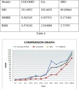
We also evaluate the value of mean magnitude relative error (MMRE) and root mean square (RMS), using the equation 9, 10 which are given as follows.
Models COCOMO GA SBO
MD 251.0953 102.6035 89.89864
MMRE 0.562165 0.207531 0.173401
[image:7.612.172.441.408.712.2]RMS 4.574342 2.924088 2.73707
VI. CONCLUSION
The Effort estimation process is based on two coefficients that is a and b according to the Boehm’s COCOMO formula. In this paper the Satin Bowerbird optimization algorithm uses the optimized value of a and b, so that estimation of effort is found near to the actual effort. In the future there may be work on the new weights estimation in the COCOMO Model by which the effort estimation can give more accurate result.
REFERENCES
[1] K. Molokken and M. Jorgensen, A Review of Software Surveys on Software Effort Estimation, In ISESE 2003. Proceedings International Symposium on Empirical Software Engineering, IEEE, pp. 223–230, (2003).
[2] B. W. Boehm, et al., Software Engineering Economics, Prentice-hall Englewood Cliffs (NJ), vol. 197, (1981).
[3] A.Sharma and D. S. Kushwaha, Estimation of Software Development Effort from Requirements Based Complexity, Procedia Technology, vol. 4, pp. 716– 722, (2012).
[4] Seyyed Hamid Samareh Moosavi, Vahid Khatibi Bardsiri,” Satin bowerbird optimizer: A new optimization algorithm to optimize ANFIS for software development effort estimation”,Engineering Applications of Artificial Intelligence 60 (2017) 1–15
[5] A.Sharma, M. Vardhan and D. S. Kushwaha, A Versatile Approach for the Estimation of Software Development Effort Based on srs Document, International Journal of Software Engineering and Knowledge Engineering, vol. 24(01), pp. 1–42, (2014).
[6] Gall,inn,ina, O. Burceva and S. Parˇsutins, The Optimization of Cocomo Model Coefficients Using Genetic Algorithms, (2012).
[7] K.Choudhary, “GA based Optimization of Software Development effort estimation”, International Journal of Computer Sci ence and Technology ,vol.1 (1),pp. 38-40,2010.
[8] A.S.Vishali, “COCOMO model Coefficients Optimization Using GA and ACO”, International Journal of Advanced Research in Computer Science and Software Engineering ,vol. 4 (1),PP.771-777,2014.
[9] L. Oliveira, “GA-based method for feature selection and parameters optimization for machine learning regression applied to software effort estimation”, information and Software Technology, vol.52,PP.1155-1166, 2010.
[10] O. Galilina, “The Optimization of COCOMO Model Coefficients Using Genetic Algorithms”, Information Technology and Management Science ,pp.45-51,2012.
[11] V. Khatibi, and D. Jawawi, “ Software Cost Estimation Methods: A Review”, Journal of Emerging Trends in Computing and Information Sciences ,vol 2 ,pp. 21-29,2011.
[12] S. M. Sabbagh Jafari, F. Ziaaddini,” Optimization of Software Cost Estimation using Harmony Search Algorithm” 1st Conference on Swarm Intelligence and Evolutionary Computation (CSIEC2016), Higher Education Complex of Bam, Iran, 2016.
[13] K.Choudhary, “GA based Optimization of Software Development effort estimation”, International Journal of Computer Sci ence and Technology ,vol.1 (1),pp. 38-40,2010.
[14] V. Khatibi, and D. Jawawi, “ Software Cost Estimation Methods: A Review”, Journal of Emerging Trends in Computing and Information Sciences ,vol 2 ,pp. 21-29,2011.