scBFA: modeling detection patterns to mitigate technical noise in large scale single cell genomics data

M E T H O D

Open Access

scBFA: modeling detection patterns to

mitigate technical noise in large-scale

single-cell genomics data

Ruoxin Li

and Gerald Quon

Abstract

Technical variation in feature measurements, such as gene expression and locus accessibility, is a key challenge of large-scale single-cell genomic datasets. We show that this technical variation in both scRNA-seq and scATAC-seq datasets can be mitigated by analyzing feature detection patterns alone and ignoring feature quantification measurements. This result holds when datasets have low detection noise relative to quantification noise. We demonstrate state-of-the-art performance of detection pattern models using our new framework, scBFA, for both cell type identification and trajectory inference. Performance gains can also be realized in one line of R code in existing pipelines.

Keywords:scRNA-seq, Dimensionality reduction, scATAC-seq, Technical noise, Gene detection, Gene

quantification, Cell type identification, Trajectory inference, Variable gene selection

Background

Single-cell genomics technologies have become a widely used technique for investigating diverse problems related to gene regulation, including the identification of novel cell types and their regulatory signatures, trajectory in-ference for the analysis of continuous processes such as differentiation, high-resolution analysis of transcriptional dynamics, and characterization of transcriptional hetero-geneity within populations of cells [1]. Of the different modalities that can be profiled, single-cell RNA sequen-cing (scRNA-seq) is currently the most mature; diverse scRNA-seq technologies are now available to cater to-wards specific applications. For instance, droplet-based methods, such as Drop-seq, currently have some of the highest throughput capture of cells and are suitable for rare cell type identification and characterization of tissue heterogeneity. The so-called full-length transcript methods are able to measure alternative splicing and se-quence individual cells more deeply, with the limitation of typically sequencing fewer cells.

scRNA-seq technologies are still rapidly evolving [2], and one of the most pressing challenges today is to ad-dress a large amount of technical noise that can drive approximately 50% of the cell-cell variation in expression measurements [3–5]. Two such expression measure-ments of interest are gene detection (the identification of the set of all genes truly expressed in a given cell) and gene quantification (the estimation of the relative num-ber of transcripts per gene and cell, also referred to as counts); the fidelity of these measurements for a given technology is termed its sensitivity and accuracy, re-spectively. Both sensitivity and accuracy vary widely be-tween scRNA-seq technologies [6], which is the result of the small quantities of RNA sequenced per cell, reverse transcriptase inefficiency, and amplification bias [5], among other features of the scRNA-seq protocols.

Independent of technology choice, scRNA-seq experi-mental design necessitates a cost trade-off between dee-per sequencing of individual cells and sequencing more cells overall. We have observed that as the number of cells sequenced increases, the average gene detection rate decreases, as does the average number of molecules sequenced per cell (Additional file 1: Figure S1), due to both choice of technology and cost trade-off. We rea-soned that when the number of unique molecules drops

© The Author(s). 2019, corrected publication 2019.Open AccessThis article is distributed under the terms of the Creative Commons Attribution 4.0 International License (http://creativecommons.org/licenses/by/4.0/), which permits unrestricted use, distribution, and reproduction in any medium, provided you give appropriate credit to the original author(s) and the source, provide a link to the Creative Commons license, and indicate if changes were made. The Creative Commons Public Domain Dedication waiver (http://creativecommons.org/publicdomain/zero/1.0/) applies to the data made available in this article, unless otherwise stated.

* Correspondence:[email protected]

1_{Graduate Group in Biostatistics, University of California, Davis, Davis, CA, USA} 2_{Genome Center, University of California, Davis, Davis, CA, USA}

too low, the signal-noise ratio of the data may be too low to make gene quantification informative [7], and therefore, downstream analyses should be adapted to primarily consider only gene detection patterns.

In this paper, we make the key observation that on scRNA-seq datasets exhibiting high technical noise, di-mensionality reduction using only the gene detection measurements is superior to the existing state-of-the-art methods that use both detection and quantification mea-surements [8,9]. We show that our new detection-based model, single-cell binary factor analysis (scBFA), leads to better cell type identification and trajectory inference, more accurate recovery of cell type-specific markers, and is much faster to perform compared to several quantification-based methods. Through simulation ex-periments, we demonstrate that our gene detection model is superior precisely when quantification noise ex-ceeds detection noise, providing a principled explanation for when and why discarding quantification estimates is advantageous. Finally, we demonstrate the superiority of our detection model in the analysis of single-cell chro-matin accessibility data, suggesting detection models may improve downstream analysis of other single-cell genomic modalities in high-throughput datasets.

Results

scBFA achieves superior performance in cell type identification across diverse benchmarks

We first hypothesized that the performance of scRNA-seq analysis tools that model gene counts (quantification) could be improved by instead modeling only the gene de-tection patterns when analyzing datasets that have a high degree of technical noise. Our intuition is that it is well established that poorly expressed genes are hard to accur-ately quantify using single-cell genomics technologies due to technical noise [10,11]. Extrapolating to an entire data-set, we then reasoned that for datasets in which technical noise leads to low gene detection and noisy quantification, modeling differences in small gene counts is challenging and prone to error, and therefore, focusing only on gene detection would be more robust.

To test our hypothesis, we developed single-cell binary factor analysis (scBFA), a method for dimensionality re-duction that only uses gene detection patterns. We com-pared scBFA against seven other approaches that model gene counts and represent the spectrum of approaches to identifying cell types within scRNA-seq datasets (see the

“Methods” section): scVI [12], SAVER [13], sctransform [14], scrna2019 [15], PCA, ZINB-WaVE [8], and scImpute [9]. scBFA is designed as a gene detection-based analog of WaVE, and so, comparison of scBFA versus ZINB-WaVE is the most direct comparison of gene detection versus quantification-based approaches. In this study, we focus on the task of dimensionality reduction, as it is a

nearly ubiquitous first step both for data visualization and analysis [16–18] and many analysis tools have been developed to address it [8,9,12,19,20]. Furthermore, pre-vious work has shown that cell type identification and di-mensionality reduction are still possible in scRNA-seq experimental designs favoring high cell counts, with low coverage per cell [4,21–23].

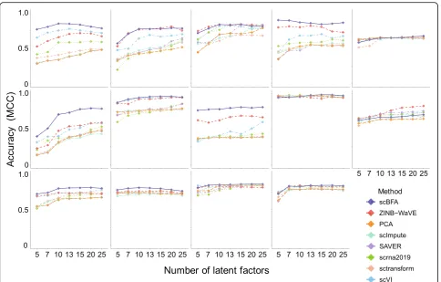
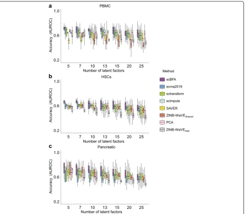
We evaluated the methods using 14 benchmark datasets for which experimentally defined cell type labels were available (Additional file1: Table S1) by first learning low dimensional embeddings, then using the embeddings to predict cell type labels in a supervised setting. When using highly variable genes (HVGs) as a gene selection criterion during data preprocessing, we found scBFA was the best, or tied for best, in 13 out of 14 benchmarks (Figs.1and2, Additional file1: Figures S2-S3). This result was robust to the selection of the hyperparameters of scBFA (Additional file1: Figure S4). Surprisingly, we found that the choice of gene selection had a significant impact on our results. Under an alternative gene selection procedure that biases towards highly expressed genes (HEGs) and yields min-imal overlap with HVG (Additional file 1: Table S2), scBFA was a top performer in only 9 of 14 of the bench-marks (Additional file 1: Figure S5).

Gene selection shapes cell type identification

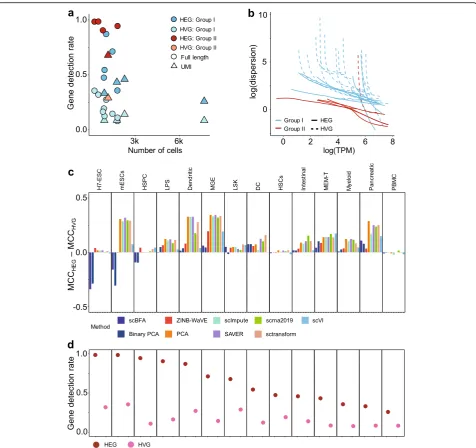
performance by modulating detection rate and dispersion We hypothesized the stark difference in performance be-tween the HVG and HEG selection criteria was due to the differences in the overall technical noise in the resulting selected gene sets. For both the HVG and HEG versions of each benchmark, we computed two indirect measures of technical noise, the gene detection rate (GDR) and gene-wise dispersion. Existing approaches to directly estimating technical noise require spike-in stan-dards [24, 25], and not all datasets we analyzed had in-corporated spike-in standards in their protocol. GDR is the average fraction of genes that are detected as expressed in a given cell. Gene-wise dispersion is intui-tively the excess variation in the gene expression ob-served beyond what is expected based on a Poisson model of sampling noise and is driven by both technical noise and biological factors of interest.

dropout noise. For scBFA, specifically, the three bench-marks for which HVG outperformed HEG correspond to the benchmarks for which HEG selection led to the high-est GDR and HVG selection led to low GDR (Fig.3c, d). The poor performance of scBFA combined with HEG se-lection can therefore be explained by the high GDR.

Across all benchmarks and gene selection criteria, we found that scBFA outperforms count-based methods for benchmarks with low GDR and high gene-wise disper-sion (Figs. 1 and 3; Additional file 1: Figure S5, group I benchmarks). This is likely because higher dispersion in-creases the noise within the gene counts, forcing count-based models and their low-dimensional embeddings to explain more outliers and noise in the data; this is par-ticularly true for count models that share variance pa-rameters across genes [8, 26]. The gene detection pattern is more robust to noise than counts because moderately to highly expressed genes are likely to be equally well detected even in the presence of technical noise. Interestingly, low GDR of a dataset in particular is associated with more sequenced cells regardless of the experimental protocol used (Additional file 1: Figure S1) and is likely a result of investigators trading off

sequencing many cells at the cost of sequencing fewer reads per cell. These results together suggest that scBFA is more appropriate for large-scale dataset analysis than quantification-based methods.

Inversely, high GDR is more typical of smaller datasets (Additional file 1: Figure S1) and yields poor perform-ance of scBFA. This is because when the GDR reaches close to 100%, every gene is detected in nearly every cell, so there is a limited variation for scBFA to capture in its embedding space. Consistent with these results, we found that the performance of scBFA decreases after im-putation (SAVER-scBFA, scImpute-scBFA) relative to before imputation (scBFA) (Additional file 1: Figure S6), in part because imputation increases GDR by imputing false-positive zero expression. On average, SAVER in-creased the GDR by 9.6% and scImpute increases GDR by 232.6%.

Balance of detection and quantification noise determines the relative performance of detection and count models We next sought to identify precisely which types of technical noise were responsible for the relative per-formance of scBFA versus the gene count models.

Fig. 1Single-cell binary factor analysis (scBFA) outperforms quantification models. Performance is measured via cross-validation of cell type classifiers

Previous studies found that sensitivity and accuracy (gene detection and quantification) can be affected differently by sequencing depth and other features of the protocols [7, 27]. We hypothesized that differ-ences in detection and quantification noise might ex-plain the performance difference between scBFA and quantification-based methods. Because technical noise is difficult to estimate in real datasets without the spike-in standards, we instead generated thousands of simulated scRNA-seq datasets that systematically vary in the relative amount of noise in gene detection and gene counts (quantification).

Our simulation framework extends the ZINB-WaVE statistical model [8] to include the parameters that sep-arately influence the noise added to either the gene de-tection pattern ðσ2_πÞ or the gene counts (σ2_μÞin the simulated datasets. We also tuned the global level of gene dispersion that drives variation in gene counts via the parameter r, which adds noise specifically to the UMI counts in the dataset and is a key parameter of many dimensionality reduction models [8, 12, 28]. Finally, we also tuned the global level of gene dropout observed in the dataset via the parameter δ, to

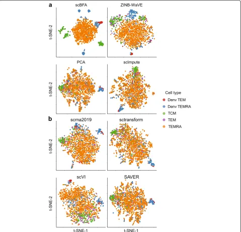
Fig. 2scBFA improves visualization of cell identity in the MEM-T benchmark of Patil et al. 2D t-SNE visualization of 10-dimensional embeddings

simulate global differences in gene detection typically observed between different protocols and technologies [6]. We first confirmed that our simulation framework gener-ates datasets with similar characteristics to real datasets. For each of the LSK, HSPC, and LPS benchmarks, we first applied the HVG selection procedure and fit the ZINB-WaVE model. Using the ZINB-ZINB-WaVE-learned parameters

and after setting our additional framework parameters

ðσ2

μ¼0:5;σ2π¼0:5;r¼1;δ¼−0:5Þ , we then

simu-lated the exact same number of cells as was in the original dataset. Upon performing dimensionality re-duction and visualization of both simulated and mea-sured cells simultaneously, we found cells clustered by cell type regardless of whether they were from the

Fig. 3Relative scBFA performance is positively correlated with dataset size and high technical noise.aGene detection rate as a function of the

real or simulated dataset (Additional file1: Figures S7-S9), confirming our simulation framework generates realistic datasets.

scBFA consistently outperforms the count-based methods in classifying cell types precisely when the gene detection noise is less than the gene count noise

ðσ2

π<σ2μÞ(Fig.4). This observation is robust to the choice

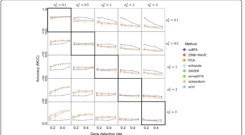
of gene dispersion parameter r(Additional file1: Figures S10-S11) and gene selection procedure (Fig.4, Additional file 1: Figures S12-S14). On real datasets, we found that scBFA performance increases as the gene detection rate decreases (Fig.3a), suggesting that in the real datasets for which GDR is low, the count noise may exceed the detec-tion noise.

scBFA mitigates technical and biological noise in noisy scRNA-seq data

We next tested each method’s ability to reduce the effect of technical variation on the learned low-dimensional embeddings by training them on an ERCC-based dataset [29] with no variation due to biological factors. In this dataset, ERCC synthetic spike-in RNAs were diluted to a

single concentration (1:10) and loaded into the 10× platform in place of biological cells during the gener-ation of the GEMs. This dataset therefore consists of a single “cell type,” with only technical variation present (since the spike-in RNAs were diluted to the same con-centration). Additional file 1: Figure S15 illustrates that both scBFA and Binary PCA yield a low-dimensional embedding with minimal variation between“cells” com-pared to the other methods, suggesting that gene detec-tion models are systematically more robust to technical noise compared to count models.

We also found that modeling gene detection patterns helps to mitigate the effect of biological confounding factors in the scRNA-seq data. For example, a common data normalization step is to remove low-quality cells for which many reads map to mitochondrial genes, as these cells are suspected of undergoing apoptosis [30]. However, finding a clear threshold for discarding cells based on mitochondrial RNA content is challenging (Additional file 1: Figure S16). We found that low di-mensional embeddings learned by count-based methods are clearly influenced by mitochondrial RNA content, but this is not true for scBFA (Additional file 1: Figures

Fig. 4scBFA outperforms quantification models when the gene detection noise is less than gene quantification noise. Rows represent different

settings of (gene) detection noise (σ2

π), and columns represent different settings of (gene) quantification noise (σ2μ). The diagonal represents simulations

where the detection noise is equal to the quantification noise (σ2

μ¼σ2π), and the plots above the diagonal represent simulations where the detection

S17-S18), suggesting that scBFA analysis of data will make the downstream analysis more robust to the inclu-sion of lower-quality cells.

scBFA embedding space captures cell type-specific markers We further hypothesized that scBFA performs well at cell type classification in high-quantification noise data because detection pattern embeddings are purely driven by genes only detected in subsets of cells such as marker genes, while this is less true for count models. Marker genes should always be turned off in unrelated cell types and always be expressed at some measurable level in the relevant cells.

To test our hypothesis, we measured the extent to which learned factor loadings capture established cell type markers on the PBMC, HSCs, and Pancreatic benchmarks, for which clear markers could be identified. For these 3 datasets, we identified 41, 43, and 73 markers, respectively, from the literature (Additional file1: Tables S3-S5). Gene selection reduced the marker sets further to 30, 24, and 43 markers for HVG and 20, 28, and 47 for HEG, respect-ively. Figure5 demonstrates that for these 3 datasets, the embeddings of scBFA are driven by cell type markers more than the quantification-based methods, despite the fact that the cell type markers are not used when learning the embeddings. These results also hold when HEG selec-tion is used instead of HVG (Addiselec-tional file1: Figure S19). An important conceptual difference between scBFA and quantification-based methods, such as ZINB-WaVE, is that scBFA treats all zero-count measurements as true observations in which a specific gene is truly not expressed in a given cell. In contrast, ZINB-WaVE and others try to statistically distinguish dropout events from true zero-count measurements. As a result, the ZINB-WaVE model has a gene detection-specific feature matrix and gene count-specific feature matrix nent, and we compared the performance of each compo-nent individually with respect to the cell type marker identification. Figure5illustrates that scBFA factor load-ing matrix outperforms both components of ZINB-WaVE, suggesting the proportion of false-positive (un-detected) zero-count measurements is relatively small and hard to infer statistically.

Trajectory inference improves with detection modeling One of the most tantalizing applications of scRNA-seq is trajectory inference for identifying changes in the gene ex-pression during continuous processes such as differenti-ation [31]. There are on the order of at least 45 methods for trajectory inference [32]. The first step to many trajec-tory inference methods is dimensionality reduction, of which PCA is a commonly used method [31]. Using a re-cent benchmark of trajectory inference methods, we iden-tified Slingshot, a top-performing method that uses

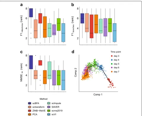
dimensionality reduction [33]. We evaluated Slingshot’s performance on a set of 18“gold standard” trajectory in-ference benchmarks after we replaced its PCA step with one of the dimensionality reduction methods we have benchmarked [32]. We found that substituting scBFA in place of PCA led to a systematically higher performance compared to the other methods (ZINB-WaVE, PCA, scImpute, SAVER, scrna2019, sctransform, scVI) (Fig. 6). These results are robust to the performance metric (Fig.6, Additional file1: Figure S20).

Detection pattern models are also superior for scATAC-seq data analysis

Several of the features of scRNA-seq protocols thought to drive technical noise are also shared among other single-cell genomic technologies, such as small starting material and amplification bias. We therefore reasoned that detection-based approaches, such as scBFA, are applicable to other types of single-cell genomic data. We measured the ability of scBFA to cluster cells into cell types using scATAC-seq datasets, which also typically produce highly sparse datasets. scATAC-seq datasets are not typically suitable for input into scRNA-seq analysis tools, because the largest values observed in scATAC-seq data corres-pond to the ploidy of the genome (e.g., two for humans). However, such sparse, small count data means that trans-formation into a detection pattern matrix suitable for in-put into a method such as scBFA will not significantly alter the input data, making scBFA potentially more generalizable than other scRNA-seq analysis tools.

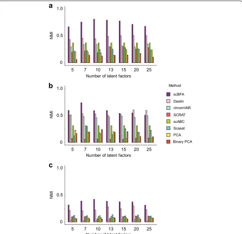
We performed dimensionality reduction and cell type classification experiments on several scATAC-seq datasets, analogous to our scRNA-seq analyses above. We benchmarked scBFA against PCA, Binary PCA, Scasat [34], Destin [35], scABC [36], chromVAR [37], and SCRAT [38]. scBFA systematically outperformed all other methods in our benchmark datasets (Fig. 7, Additional file 1: Figures S21-S24). An important ad-vantage of scBFA over the other scATAC-seq methods is that only scBFA can systematically adjust for the cell-level covariates such as QC measurements (e.g., cell cycle stage) and batch effects. In contrast, other methods, such as Scasat, are unable to remove batch effect in all features since Scasat removes batch effects through removing batch-specific loci, which can be confounded with cell type-specific loci de-pending on the experimental design. Methods such as Binary PCA cannot directly regress out continuous covariates.

occasionally exceeding one million cells, computational efficiency of scRNA-seq analyses becomes challenging as ideally these tools could be run on local machines. We therefore benchmarked methods in terms of their speed of computation. In our comparisons, we also in-cluded a fast approximation of scBFA, which we term Binary PCA. Binary PCA is easy to implement in one line of R code (we simply transform the gene counts into the gene detection patterns as a preprocessing step before use of PCA) and provides immediate benefits over standard PCA and other methods with respect to cell type identification (Additional file 1: Figures

S25-S26). We found that Binary PCA is tied for the fastest of all methods, while scBFA is still faster than several com-peting count-based methods (Additional file 1: Figure S27). More specifically, scBFA is a median of ten times faster than ZINB-WaVE. The difference in the execution time between scBFA and ZINB-WaVE is due primarily to the additional burden of modeling gene quantification be-cause the scBFA model structure and parameter learning algorithm were designed to match the gene detection pat-tern component of ZINB-WaVE as closely as possible. This suggests that gene detection models may help ana-lysis tools scale to larger datasets in the future.

Fig. 5scBFA is better informed by cell type markers than quantification models. Each latent factor learned from each method was evaluated

Discussion

Our primary result is that when the count (quantifi-cation) noise is relatively high in a dataset as is typ-ical in larger datasets, the effects of this noise on the downstream analysis can be mitigated by modeling detection patterns instead of counts. The improve-ment in the performance of scBFA over ZINB-WaVE in this regime (Figs. 1 and 3) is particularly inform-ative because the ZINB-WaVE model has two compo-nents: one that models gene detection and the other that models gene counts (quantification). The model structure and parameter learning algorithm of scBFA are designed to match the gene detection component

of ZINB-WaVE as closely as possible, making the dif-ference in their performance primarily due to whether gene quantification (ZINB-WaVE) or gene detection (scBFA) is modeled.

We show that as the number of cells sequenced in-creases within a dataset, the technical noise in the data (as measured indirectly by the gene detection rate and gene-wise dispersion) and the relative performance of scBFA generally increase as well. Because many scRNA-seq applications benefit from higher numbers of se-quenced cells, there is a steep upward trend of scRNA-seq dataset sizes, with some recent datasets containing nearly a million cells [2]. Our results therefore suggest

Fig. 6scBFA leads to the most improvement in trajectory inference performance of Slingshot.a_–cSlingshot was modified by replacing the PCA

that it is increasingly important that next-generation scRNA-seq analysis tools exploit the advantages of gene detection-only modeling in order to mitigate the effects of technical noise within the data. Also, given the influ-ence of technology and protocol choice on technical noise in scRNA-seq data [6], our results imply that fu-ture scRNA-seq tools could be designed to take advan-tage of the specific noise structure implied by different scRNA-seq protocols, as opposed to being relatively protocol-agnostic as they are today.

While it is challenging to measure technical noise in real datasets, we show that the gene detection rate and

gene-wise dispersion are easily calculated and serve as good proxies for measuring technical noise. In our re-sults, we found that the performance of scBFA exceeds that of gene count analysis tools in cell type classifica-tion when the gene detecclassifica-tion rate falls below 90% and dispersion estimates are high, therefore providing the community with a general guideline for when detection-based tools, such as scBFA, should be used instead of quantification-based tools. Our R package also has imple-mented a function, diagnose, to assist users in determining whether scBFA is appropriate for their data. Our results are also consistent with previous work that shows tasks,

Fig. 7scBFA more accurately recovers cell type identity in scATAC-seq datasets. Clustering accuracy (NMI) of each scATAC-seq method trained

such as dimensionality reduction, cell type identification, and abundance estimation, can be performed successfully when individual cells are sequenced to shallow depth [4,

21–23] and further provide a complementary analysis ap-proach suitable for these datasets with low per-cell se-quencing depth.

There is a plethora of data normalization methods that have been, and continue to be, designed to decrease tech-nical noise within and across cells, in order to better per-form both gene detection and quantification, and to make these quantities comparable across cells (see [5,39,40] for an overview). The challenge we address here is not miti-gated by data normalization methods; however, as we argue that when the number of UMIs sequenced per cell decreases drastically, gene quantification information spe-cifically is not present (or useable) in the data, which is a problem that data normalization cannot mitigate. Data normalization works complementarily to gene detection pattern analysis however, as illustrated by our use of data normalization before gene detection modeling in this work. Our results also imply that models that statistically dis-tinguish dropout events from genes truly not expressed in a cell may be less fruitful for large datasets. Many gene count-based methods [9, 24, 41] model zero counts as a mixture of genes truly turned off (biological signal) and genes that are truly expressed but not detected due to technical artifacts from the experimental protocol (tech-nical noise) [41]. On the contrary, gene detection pattern methods, such as scBFA, treat all zeroes as a biological sig-nal, a key feature motivated by the observation that zero measurements driven by technical noise tend to occur for genes that are poorly expressed [10,11]. The superior per-formance of scBFA when the gene detection rate is low suggests that for these datasets, there is not enough infor-mation in the gene counts to reliably detect technical dropout events, and therefore, traditional mixture model-ing can be unhelpful for high-throughput datasets where gene detection rates are low overall.

The success of modeling gene detection patterns in scRNA-seq is not tied to a specific model structure. The performance improvement of scBFA over ZINB-WaVE, and Binary PCA over PCA, demonstrates our results hold across multiple model structures and loss functions. In both cases, not only do we observe per-formance gains for large scRNA-seq datasets, but there is also a substantial speed improvement because detection modeling avoids complex parametric model-ing of gene counts, makmodel-ing detection models scalable to larger datasets. Within the class of gene detection-based models, Binary PCA provides a moderately ac-curate but much faster and simpler implementation scheme that can be achieved in one line of code, making our results readily achievable by the current analysis pipelines.

A surprising finding was that HEG gene selection led to a systematically better cell type identification for every tested method in almost all datasets, compared to HVG selection (Fig. 3c). HVG selection anecdotally is the standard criterion upon which variable genes are typic-ally selected during preprocessing [42], suggesting at least for cell type identification, HEG selection may lead to improved performance regardless of the method used. While single-cell genomic data from different modal-ities, such as scATAC-seq, have similar data structure as scRNA-seq data, the analysis tools and pipelines devel-oped to date for those two technologies are largely mu-tually exclusive. Here, we show that scBFA generalizes to other single-cell genomic modalities and outperforms the existing methods for cell type identification for scATAC-seq datasets as well, even those that take ad-vantage of auxiliary data such as transcription factor mo-tifs and distance to transcription start sites [35]. We expect our results to generalize to other single-cell gen-omic modalities such as single-cell methylation or his-tone modification data.

Methods

Single-cell binary factor analysis (scBFA) model

scBFA is available as an R package on Bioconductor at

https://bioconductor.org/packages/devel/bioc/html/scBFA .html, as well as on GitHub (https://github.com/quon-tita tive-biology/scBFA). The main function to run scBFA is scBFA().

In our notation below, matrices are represented by upper case bold letters, vectors by lower case bold ters, and numeric constants as upper case non-bold let-ters. Square brackets also indicate a matrix, though represented as a series of column vectors. A matrix sub-script with round brackets indicates the index of the cor-responding column vector.

The schematic of our single-cell binary factor analysis (scBFA) model is shown in Additional file 1: Figure S28. The input data to scBFA consists of two matrices,O and X.Ois a matrix of counts, consisting ofGfeatures (genes in the case of scRNA-seq data, or loci in the case of scATAC-seq data) measured in each ofNsamples (cells). From the input dataO, we compute a matrixB, whereBij

represents the detection pattern observed for celli (i= 1,

…,N) and feature j (j= 1,…,G). For scRNA-seq inputs, Bij= 1 whenOij≥1, otherwiseBij= 0. Therefore,Bij= 1

in-dicates that at least one read (or UMI) maps to genejin celliand therefore suggests gene expression. Similarly, for scATAC-seq input data, Bij= 1 when Oij≥1, in other

words, when at least one read maps to locusjin celli(and therefore suggests locus accessibility), otherwise Bij= 0.

…,xN]Tis aN×Ccell-level covariate matrix that enables

correction forC observed nuisance factors such as batch effects or other cell-specific quality control measurements. If there are no such cell-level covariates that need to be ad-justed for,Xis the null matrix by default.

The intuition behind scBFA is that it performs dimensionality reduction to explain the high-dimensional detection pattern matrix B by estimating two lower-dimensional matrices: a N × K embedding matrixZ= [z1,z2,…,zN]T,and aK×Gloading matrix

A= [a1, a2,…, aG]. Here,Kis the number of latent

di-mensions used to approximate Bij, where whereK≪G.

ui and vi and represent the ith cell-level intercept and

jth feature-specific intercept, respectively. u is therefore a vector of lengthN, and v is a vector of length G. For scRNA-seq, for example, we expect u and v will impcitly model the variation of gene expression caused by li-brary size. µij is the mean of the Bernoulli distribution

governing whether featurejis detected in cellior not. Formally, scBFA is defined by the following model:

logitðμi jÞ ¼xTiβjþzTiajþuiþvj

PðB;A;Z;β;X;u;vÞ ¼Y

i;j

Bernoulli Bijjμij;A;Z;β;X;u;v

We train the scBFA model by optimizing the following penalized likelihood function:

fðB;A;Z;β;X;u;vÞ ¼ X_i;j lnP B ij;A;Z;β;X;u;v

h i

−ϵ1k kA 22−ϵ2k kZ 2 2−ϵ3k kβ

2 2

Here, ϵ1, ϵ2, and ϵ3 are the tunable parameters that

control the regularization of the model parameters, where by default ϵ1¼ϵ_G0;ϵ2¼_Nϵ0, ϵ3¼ϵ_G0, and ϵ0= max {

N,G}. The optimization is carried out using the L-BFGS-B optimization routine available in the R optim() function. After completing the optimization, we orthog-onalize Z and A using the orthogonalizeTraceNorm() function available in the ZINB-WaVE [8] package.

Binary PCA model and calculation of the gene detection pattern matrix

Binary PCA describes our fast approximation to scBFA by simply running PCA, with the exception of converting the input count matrix into a detec-tion matrix by converting non-zero values to one. We implemented Binary PCA through the addition of a single line of R code. Suppose that countMatrix is the name of the matrix in R that stores, for ex-ample, the UMI counts for each gene in each cell. To run Binary PCA, we first convert the countMa-trix into the gene detection pattern macountMa-trix before

running PCA via the R command:

countMatrix[which(countMatrix>0)] <- 1

We then call PCA using the following command in R:

PCA_results <- prcomp(countMatrix, center=TRUE, scale.=FALSE);

Note that typically, scale is set to TRUE when calling PCA. For Binary PCA, we set it to FALSE because the variance in gene detection is potentially associated with cell types (e.g., genes with higher detection variance are more likely to be marker genes, and therefore should contribute more to the embedding).

Execution of scRNA-seq analysis methods

We compared scBFA against scVI [12], SAVER [13], sctransform [14], scrna2019 [15], PCA, ZINB-WaVE [8], and scImpute [9]. These seven methods were selected to represent diverse classes of approaches to scRNA-seq data analysis, including dimensionality reduction methods (PCA, ZINB-WaVE, scVI), preprocessing approaches that can be applied before dimensionality reduction (sctrans-form, scrna2019), and imputation methods that can be ap-plied before dimensionality reduction (SAVER, scImpute). Of the dimensionality reduction methods, PCA was chosen because of its implementation in popular packages such as Seurat [42], and scVI [12] is a leading deep learning-based dimensionality reduction method. ZINB-WaVE was chosen specifically because it is a recently de-veloped method, and scBFA is designed as a gene detection-based analog of ZINB-WaVE; therefore, com-paring scBFA with ZINB-WaVE is the fairest comparison of gene detection versus quantification-based approaches.

We ran most of the scRNA-seq analysis methods with their default parameter settings, with the exception of scVI and scrna2019.

For the simulated datasets, given the large number of scenarios tested, we fixed the learning rate to be 0.001 and number of iterations to be 2000.

scrna2019 is a method developed to perform feature selection and GLM-based factor analysis on scRNA-seq [15]. The scrna2019 R package (obtained on May 6, 2019, fromhttps://github.com/willtownes/scrna2019) of-fers both a GLM factor analysis model and a corre-sponding deviance score approximation. We used the deviance score approximation instead of the GLM framework for our experiments because several bench-marks required batch effect correction, which should be addressed using the deviance score approximation as per scrna2019’s authors’recommendations [15]. Also, at the time of the writing of this paper, the GLM implementa-tion produced errors for three of our datasets that pre-vented us from completing our experiments.

Execution of scATAC-seq analysis methods

We compared scBFA against PCA, Binary PCA, Scasat [34], Destin [35], scABC [36], chromVAR [37], and SCRAT [38]. Scasat and Destin are scATAC-seq analysis tools primarily designed to identify cell types and differential ac-cessibility analysis. Both methods treat dimensionality re-duction as a prior step before further clustering distinct cell types. Scasat’s embedding space is learned by perform-ing multidimensional scalperform-ing (MDS) on a cell-cell Jaccard similarity matrix computed from a binarized chromatin ac-cessibility matrix. Destin developed a weighted principal component analysis approach using distance to transcrip-tion start sites and reference regulomic data. scABC is an unsupervised clustering tool of single-cell epigenetic data and performs multi-stage clustering based on the input chromatin accessibility matrix directly. chromVAR aggre-gates motif position weight matrices (PWM) and chroma-tin accessibility to uncover cell populations and identify motifs associated with cell type-specific variation. SCRAT summarizes several distinct regulatory genomic data (in-cluding prior established gene sets and transcription factor binding motif sites, among others) to identify distinct cell populations from single-cell genomic data.

For SCRAT, we used the regulatory activity feature list provided by SCRATsummary() as the default input fea-tures. In addition, we also input the BED files correspond-ing to the scATAC-seq data as a custom feature as suggested by the SCRAT authors [38], which we found to improve the performance.

Quantifying the effect of imputation on scBFA

We compared the performance of scBFA before and after imputation on our 14 benchmark datasets under HVG se-lection. We tested two state-of-the-art imputation methods, SAVER [13] and scImpute [9]. SAVER estimates

library size-normalized posterior means of gene expres-sion levels (^λij), which are inappropriate for input into

scBFA because they are not sparse. We therefore sampled counts from SAVER’s generative model as follows:

Oij∼Poisson si^λij

where^λijis SAVER’s imputed expression level andsiis the library size for cell i divided by the mean library size across cells [13]. We generated five separate count matri-cesOijbased on the SAVER estimates ^λij. For scImpute, we used its imputed gene counts matrix directly as input for scBFA.

Selection of representative datasets to measure gene detection rates

We obtained a total of 36 scRNA-seq datasets from which we calculated gene detection rates as a function of the num-ber of cells in each dataset (Additional file 1: Figure S1). We obtained these datasets from two sources, the conquer database [43] and the Gene Expression Omnibus (GEO) [44]. For GEO, we used the search term“((‘single cell rna-seq’ OR ‘single cell transcriptomic’ OR ‘10X’ OR ‘single cell transcriptome’) AND Expression profiling by high throughput sequencing[DataSet Type]) AND (Homo sapiens[Organism] OR Mus musculus[Organism]),”sorted all datasets by size, then selected a similar number of datasets from both the top and bottom of the list (Additional file 1: Table S7).

Computing mean and dispersion curves

therefore chose the fitted dispersion estimates to gener-ate Fig.3b.

Benchmarking dimensionality reduction methods for scRNA-seq

We evaluated each dimensionality reduction method by how well their low dimensional embeddings discriminate experimentally defined cell types. For each dataset and method tested, we first performed dimensionality reduc-tion on the entire dataset to obtain an embedding matrix representing each cell inKdimensions (the matrixZ de-scribed in the scBFA methods section). We then per-formed fivefold cross-validation in which we trained a non-regularized multi-level logistic classifier on the training embeddings from each method using the a priori known cell type labels, then used the model to predict cell type labels for the test embeddings. For every prediction, using the known cell type labels, we com-puted a confusion matrix and the corresponding Mat-thews’ correlation coefficient (MCC) as a measure of classification accuracy. MCC was calculated using the R package mltools. We repeated the fivefold cross-validation a total of 15 times and reported the mean classification accuracy as the final accuracy.

MCC¼ TPTN−FPFN

ðpffiffiffiffiffiffiffiffiffiffiffiffiffiffiffiffiffiffiTPþFPÞ ðpffiffiffiffiffiffiffiffiffiffiffiffiffiffiffiffiffiffiffiTPþFNÞ ðpffiffiffiffiffiffiffiffiffiffiffiffiffiffiffiffiffiffiffiTNþFPÞ ðpffiffiffiffiffiffiffiffiffiffiffiffiffiffiffiffiffiffiffiffiTNþFNÞ

In our analysis of the ERCC dataset, we used a differ-ent evaluation metric because each “cell” represents technical replicates of the spiked-in RNA diluted at a constant ratio (10:1). Under the assumption that the only variation between“cells” is due to technical factors, we therefore used averaged within-group sum of squares (AWSS) to measure how the low-dimensional embed-ding learned by each method captured such homogen-eity. Given an Nby K embedding matrixZ, AWSS was calculated as follows:

W ¼Z−Z

AWSS¼trace W T_W

N−1

Here,Zis anNbyKmatrix for which every row is the column mean ofZ.

Benchmarking cell type identification methods for scATAC-seq

We benchmarked scBFA against existing scATAC-seq analysis tools by evaluating their ability to correctly clus-ter cell types. We used a different evaluation scheme from that used for the scRNA-seq experiments because one of the existing methods (scABC) does not produce low-dimensional embeddings and instead outputs cluster labels. The methods Scasat and Destin both provide

cluster labels directly from their analysis pipeline. For scBFA, PCA, Binary PCA, chromVAR, and SCRAT, we clustered cells based on the learned embedding matrices using R’s built-in hierarchical clustering function hclust() with Wald’s distance. We compared the accuracy of the clustering results from each method using the metrics normalized mutual information (NMI) and Adjusted Rand Index (ARI), computed using the R package aricode.

Simulation of scRNA-seq data

A variation of the ZINB-WaVE model was used to simulate scRNA-seq datasets and is defined as follows (Additional file 1: Figure S29):

zμð Þi∼N ^zi;σ2_μIK

zπð Þi∼N^zi;σ2πIK

logit πij ¼ zTπð Þia^πð Þj þu^πð Þi þ^vπð Þj−δ

log μij ¼ zTμð Þia^μð Þj þ^μμð Þi þ^vμð Þj

Πij∼Bernoulli(πij)

Oij

¼0 ifΠij¼1 ∼NB μ_ij;r

ifΠij¼0

(

To keep the consistency of the notation, the parameters we used abovefZ^;A^μ;A^π;u^μ;u^π;^vμ;^vπgrespectively

cor-respond to the parameters fW^;αμ^ ;^απ;γ^_π;γ^_μ;^β_μ;β^_πg used in the original ZINB-WaVE paper. In the first step of our simulations, all parameters with a hat accent are set a priori by fitting the ZINB-WaVE model using its R pack-age [8] on a single scRNA-seq dataset in order to use real-istic parameters for our simulation. The remaining parametersfδ;σ2_μ;σ2_π;rg are then systematically varied in our simulations to determine their effect on downstream dimensionality reduction methods. Oij denotes the gene

counts for cell iand featurej. As is described in the ori-ginal ZINB-WaVE paper, Z^ ¼ ½^z1;^z2;…;^zNT is aN×K

embedding matrix, while A^μ¼ ½a^μð1Þ;^aμð2Þ;…;^aμðGÞ and ^

Aπ ¼ ½a^πð1Þ;^aπð2Þ;…;a^πðGÞ are the correspondingK×G

regression coefficient matrices for the negative binomial and Bernoulli distributions governing the gene count and detection components, respectively. The output of the Bernoulli distribution is the latent variableΠij, which

de-cides whether a gene is detected (in which case the ob-served value Oij is sampled from a negative binomial

distribution), or not detected. u^μ and u^π areN× 1

gene-specific intercepts for the count matrix and detection matrix, respectively. The number of latent dimensions K used to generate the gene expression values was fixed at 5, and we used a total of 2000 highly variable genes as in the original dataset. The LPS dataset does not provide any cell-level covariates, so in these simu-lations, there are no cell- or gene-wise covariate matrices. For quality control purposes, we filtered out genes that are expressed in fewer than 1% of the cells and then filtered out cells in which less than 1% of genes are expressed.

The distinction between our simulation framework and ZINB-WaVE is that ZINB-WaVE maintains the same cell embedding space Z^ across both the gene detection and count spaces. In contrast, our frame-work relaxes this constraint by introducing individual embeddings Zπ and Zμ that are close to Z^. Formally,

Zπand Zμ are N×K embedding matrices for the gene

detection and count spaces, respectively. Each row i of Zπ and Zπ are sampled from respective

K-multi-variate Gaussian distributions with the same mean de-fined by ^zi and spherical variance parameters σ2_π and σ2

μ, respectively.

In our simulations, we varied the simulation parame-tersfδ;σ2

μ;σ2π;rgas follows. To influence the total

num-ber of gene counts detected (total detection rate), we set δ∈{−2,−0.5, 1, 2.5, 4}. To influence the variance in the gene detection and count embedding spaces, we set σ2

π;σ2μ∈f0:1;0:5;1;2;3g. Finally, we varied the common

gene dispersion parameterr∈{0.5,1, 5}. In total, the num-ber of unique parameter settings we used to simulate scRNA-seq data is 5 × 5 × 5 × 3 = 375. For each of those scenarios, we simulated 3 replicates, resulted in 375 × 3 = 1125 datasets.

Quality control of scRNA-seq data

For each scRNA-seq dataset tested, we performed a standardized quality control process. We first re-moved cells for which mitochondrial genes accounted for over 50% of the total observed counts. Then, we filtered out genes that are expressed in fewer than 1% of cells and removed cells whose library size (total read or UMI count) was less than one-eighth quantile of all cell library sizes. One exception is the MEM-T cell dataset, where we removed an extra 361 cells from the batch labeled “subject16” to remove batches that were confounded with cell types.

Preprocessing of scATAC-seq data

We followed the scATAC-seq pipeline for processing and aligning reads used by the Destin method [35], obtained from GitHub at https://github.com/urrutiag/ destin on April 22, 2019. This preprocessing pipeline

yielded 2779, 576, and 960 BAM files for GSE96769 [45], GSE74310 [46], and GSE107816 [47], respect-ively. These BAM files form the initial input of Des-tin, scABC, and SCRAT. The input chromatin accessibility matrix for chromVAR and Scasat was then obtained from Destin’s preprocessing pipeline directly.

For GSE96769, we only kept cells and genomic loci that are used in the original paper’s analysis. The in-dices for genome loci and cells that passed quality control are supplied in the supplementary files of the original paper. Beyond that, we selected a subset of frozen cells from five patients, excluding patient BM0106, and a subset of pDC cells from patient BM1137 to keep as many samples as possible while removing the part of the batches confounded with cell types. This enabled us to construct a design matrix to correct for patient-specific effects. We fur-thermore excluded cells that are labeled as unknown by the original author.

For each scATAC-seq dataset tested, we only kept genomic loci that are accessible in at least 1% of cells and then removed cells with a total number of ac-cessible sites that deviates more than 3 standard er-rors to the mean (in either direction) across all cells. The number of retained cells used as input in our downstream analysis was 1358 for GSE96769, 572 for GSE74310, and 929 for GSE108716. We found that SCRAT and chromVAR’s preprocessing pipeline gen-erated NA values, and so for these tools, we filtered out additional cells. For SCRAT, this yielded 1375 cells for GSE96769, 534 cells for GSE74310, and 815 cells for GSE108716. For chromVAR, this yielded 1358 cells for GSE96769, 529 cells for GSE74310, and 811 cells for GSE108716.

Defining cell type labels in benchmark datasets

were required to pass both scRNA-seq-specific filters (minimum of 800 reads) and ADT-specific filters (mini-mum of 50 ADT counts).

Normalization of scRNA-seq data

For each method, we also normalized cells to control for differences in library size. For PCA, we normalize the counts by setting O~ij¼ logðOciijþ1Þ, where O~ij is the normalized gene count for cell i and gene j, Oij is the

original gene count for celli and genej, and ci¼PjOij

is library size for cell i. ZINB-WaVE directly accounts for library size via their cell-specific intercept. For scIm-pute, we used the total number of imputed counts per cell as their corresponding library size and normalized in the same way as PCA. For scBFA, we estimated the feature-specific intercepts and cell-specific intercepts to implicitly model the effect of library size. SAVER uses the library size divided by the median library size across all cells to adjust for cell size. sctransform uses the log of the library size in its model. scrna2019 outputs a transformed deviance score matrix that does not depend on library size as input.

Normalization of scATAC-seq data

For PCA, we performed a log transformationO~ij¼ logð

Oijþ1Þ to adjust the counts within scATAC-seq, where

Oij is the original read count for cell i and locus j. For

scBFA, Scasat, Destin, scABC, Binary PCA, chromVAR, and SCRAT, no extra normalization was applied.

Gene selection in scRNA-seq data

Highly variable genes (HVG) selection was performed to identify the most overdispersed genes, that is, genes that exhibit more variance than expected based on their mean. The HVG selection was performed using the FindVaria-bleFeatures command implemented in Seurat 3.0. By de-fault, Seurat selected the top 2000 genes. Highly expressed gene (HEG) selection was performed to identify the genes that exhibit the highest variance across cells, regardless of their mean, and is therefore expected to capture genes with higher mean expression compared to HVGs. To identify HEGs, we calculated the gene-specific variance in the gene count space and select the top 2000 genes to make the set size comparable to HVGs.

The gene detection rate (the average fraction of cells in which a gene is detected as expressed) and gene-wise dis-persion of each dataset calculated in Fig. 3b is based on these 2000 most variant genes under both the HVG and HEG selection criteria. For the timing experiment, we only selected the top 1000 genes under the HVG criterion for computational speed.

Batch effect correction

For both scRNA-seq and scATAC-seq datasets, we per-formed two types of batch effect correction, depending on how the cell types are distributed across the batches in the dataset. For datasets where all cell types are represented in all batches (e.g., replicates, patients), such as the HSC dataset, we used those cell-level covariates to define the N×C design matrix X (see the scBFA model details above). For ZINB-WaVE, scBFA, and scVI, we regressed X out within the model structure. Since PCA does not offer a framework to regress out nuisance factors, we first regressedXdirectly from the normalized countsO~ij using

a linear model. We then applied PCA on the residual matrix and obtained the corresponding embeddings and factor loading matrix. For Binary PCA, scImpute, SAVER, sctransform, and scrna2019, we also regressed outXfrom the binary entries and imputed values separately, then used the residual matrix in the same way as for PCA.

For other datasets (MEM-T, Pancreatic, MGE in scRNA-seq, and GSE96769 and GSE74310 in scATAC-seq), some batches were missing a subset of cell types, resulting in a design matrixXthat cannot be directly used to estimate all batch effects. In this scenario, our strategy for modifying the dataset to address batch effects is as follows. Note that we use the same parametrization used to define the scBFA model earlier, except that we define a new ob-servation matrix M as a N×G matrix, where observa-tions can either correspond to measured expressed levels O, inferred binary detection pattern B, or im-puted read counts. Except for minor differences in parameterization, the GLM-based dimensionality re-duction methods scBFA and ZINB-WaVE can be summarized in the following framework, where g is the link function, P is a probability measure, and μ is the expectation over the probability measure. In the case of ZINB-WaVE, P is a zero-inflated negative bi-nomial distribution. In the case of scBFA, P is a Ber-noulli distribution.

g μij ¼ xTi βjþzTi ajþuiþvj

Mij∼P μij

We first identify the largest subset of cell types that are represented in all batches within a given dataset. De-fine Msub as the submatrix of N′ observations (N′<

N) corresponding to this subset of cell types and simi-larly define the submatrices Xsub, Zsub, Asub and usub,

M_subi0

;j

ð Þ∼P g−1 xTsubð Þi0 βjþzTsubð Þi0 ajþusubð Þ þi0 vj

^

βlearns the variance induced by different batches only. Then, we use β^ as a plug-in estimate of β, and per-formed each dimensionality method on the full dataset to obtain estimates of all other parameters. Note since both ZINB-WaVE and scBFA regularize their coefficient matrix β, Xsub and X are both standardized. For PCA,

scImpute, SAVER, sctransform, scrna2019, SCRAT, and chromVAR, we used a similar strategy to obtain ^β by using linear regression to regress out Xsub from the

ob-servation matrix corresponding to the largest subset of cell types represented in all batches. Then, we calculated the residualsRij=Mij−XβTon the full dataset withβ¼^β

fixed and performed PCA on the residual matrix R. For scVI, we were unable to modify the model framework to adjust for batch effects when they were confounded with cell types, as was the case in MEM-T, Pancreatic, and MGE. Therefore, we measured the scVI performance when we did not correct for batch effect, as well as when we per-formed naïve batch effect correction ignoring the con-founding, and then reported the best performance for scVI.

Scasat handles batch effects through the removal of batch-specific loci. However, for datasets GSE96769 and GSE74310, the batch effect is confounded with cell types. Therefore, we ran Scasat without batch effect correction because batch-specific loci would be indistinguishable from cell type-specific loci. Destin and scABC cannot ad-just batch effect on their own, and so we ran them without batch effect correction on these two datasets.

Identification of marker genes

We evaluated the extent to which the inferred dimen-sions for each method recover known marker genes (Fig.

5). For each method, we first obtained the K×Gfactor loading matrix indicating which genes are contributing to each of theK factors. Then, for every loading matrix and given number of factors, we ranked the absolute value of each gene in each factor and calculated the area under the receiver-operator curve (AUROC) to measure the extent to which the known marker genes contribute more to a factor than expected by chance.

Note that ZINB-WaVE has two loading matrices corre-sponding to the gene detection and gene count compo-nents, respectively, and therefore appears twice in Fig.5. In ZINB-WaVE,πijmodels whether a gene has been detected

or not, andμijmodels the mean for the read counts under

negative binomial distribution. As in the previous section, we used the parameters fZ^;A^μ;A^π;u^μ;u^π;^vμ;^vπg to

re-place the parametersfW^;^αμ;απ^ ;^γ_π;^γ_μ;β^_μ;^β_πgused y:

logit πij ¼ zT_πð Þ_iaπð Þj þxT_i β_πð Þ_j þuπð Þi þvπð Þj

log μ_ij ¼ zT_{μð Þi} a_μð Þ_j þxTi βμð Þj þuμð Þi þvμð Þj

The loading matrixaπthat models the gene detection

component (π) is denoted asZINB-WaVEdropout, and the

loading matrix aμ that models gene counts is denoted ZINB-WaVEmean.

Trajectory inference

To evaluate the performance gains of scBFA in the con-text of trajectory inference, we used a recently published platform, dynverse, for which “gold standard” scRNA-seq datasets were already obtained and preprocessed, and scripts and performance metrics have already been defined to evaluate trajectory inference [32]. Gold stand-ard datasets refer to those datasets in which experimen-tal (non-computational) methods were used to annotate a dataset with trajectory information such as cell type clusters (milestones) and connections between cell type clusters (milestone networks). From the 27 datasets available on June 12, 2019, that met this gold standard status and were real (not synthetic), we filtered out data-sets that had less than 170 cells, yielding a total of 20 benchmark datasets. As with our previous experiments, we used the HVG selection criterion to identify the top 2000 varying genes for dimensionality reduction.

Our strategy for benchmarking trajectory inference was to identify an existing, top-performing trajectory in-ference method that also uses dimensionality reduction in its pipeline then replace that dimensionality reduction step with one of the methods we tested in our study. The dynverse paper identified Slingshot as a top per-former [32]. To evaluate scBFA and the other methods, we substituted the PCA step of Slingshot with each di-mensionality reduction method (scBFA, ZINB-WaVE, PCA, scImpute, SAVER, scrna2019, sctransform, scVI) and used dynverse to measure the performance of each modified version of Slingshot. The number of input la-tent dimensions was set to 10. Because the Slingshot im-plementation throws NA in cases where it is uncertain of the assignment of cells to a particular lineage, we re-moved two datasets from further evaluation because the number of NAs produced prevented calculation of the performance metrics (germline-human-both_guo.rds, mESC-differentiation_hayashi.rds). For each of the 18 benchmarks (Additional file 1: Table S8), we used dyn-verse to compute three performance metrics with respect to the experimentally gathered trajectory infor-mation: F1milestones, F1branches, and NMSElm. F1milestones

measures the similarity between clustering membership of two trajectories. F1branchescompares the similarity

be-tween the assignment of two branches. NMSElm is a

inferred trajectory predicts the position of the cell in the ground truth trajectory under linear regression. Larger values of F1milestones, F1branches, and NMSElmcorrespond

to better performance. We obtained F1milestones,

F1branches, and NMSElmvia dynverse’s calculate_mapping

and calculate_position_predict functions within the dyneval package and converted raw values to ranks for Fig. 6. The wrapper function to obtain the results from Slingshot is adapted from the internal function https:// github.com/dynverse/ti_slingshot/blob/master/package/R/ ti_slingshot.R.

Visualization

After we obtain the embedding matrix from every method, we use the t-distributed stochastic embedding [49] method to project the embedding matrix onto two dimensions for visualization as a scatterplot. In all visu-alizations, the number of factors used as input to t-SNE in each visualization is 10.

Timing experiments

In the timing experiment (Additional file1: Figure S27), we randomly subsampled 1k, 10k, 50k, and 100k cells from the 1.3 million 10× brain cell dataset from E18 mice and recorded the single-core execution time (in seconds) of all methods (PCA, ZINB-WaVE, scImpute, SAVER, sctransform, scrna2019, and Binary PCA) on the same machine. Due to the non-convex nature of ZINB-WaVE’s objective function and different optimization scheme, we cannot strictly match the con-vergence criterion of ZINB-WaVE to scBFA. Therefore, we use the same number of iterations for each method that was used to generate the results in Fig. 1. Because scImpute requires specification of the number of cell clusters, we set the number of cell clusters to seven, similar to a previous study [50] that used seven as an underestimate of the true number of cell types.

Additional files

Additional file 1:Contains supplementary figures and tables,

Figures S1_–S29.,Tables S1_–S8.(DOCX 3090 kb)

Additional file 2:Review history. (DOCX 3950 kb)

Acknowledgements

Not applicable.

Review history

The review history is available as Additional file2.

Authors’contributions

RL and GQ conceived the study, analyzed and interpreted the data, and wrote the manuscript. RL wrote the code for scBFA. Both authors read and approved the final manuscript.

Funding

This project has been made possible in part by grant number 2018-182633 from the Chan Zuckerberg Initiative DAF, an advised fund of Silicon Valley Community Foundation. Funding was also provided by NSF CAREER award 1846559 to GQ.

Availability of data and materials

The source code implementing scBFA is available on a Bioconductor at

https://bioconductor.org/packages/devel/bioc/html/scBFA.html, as well as in a GitHub repository athttps://github.com/quon-titative-biology/scBFA[51]. scBFA is released under Apache License 2.0.

All datasets analyzed in this study with accession numbers and references are included in the published article and Additional file1. Benchmark datasets used for cell type identification in scRNA-seq are GSE48968 [52], GSE104157 [53], GSE100426 [54], GSE62270 [55], GSE106540 [56], GSE81076 [57], GSE100866 [48], GSE89232 [58], GSE123025 [59], GSE94383 [60], GSE100037 [61], GSE81682 [62], E-MTAB-2805 [63], and SRP073808 [64] (Additional file 1: Table S1). Benchmark datasets used for cell type identifica-tion in scATAC-seq are GSE96769 [45], GSE74310 [46], and GSE107816 [47]. Benchmark datasets used for trajectory inference in scRNA-seq are GSE59114 [65], E-MTAB-2805 [63], GSE60781 [66], GSE86146 [67], GSE70240 [68], GSE70243 [68], GSE70244 [68], GSE70236 [67], E-MTAB-3929 [69], GSE52529 [16], GSE74596 [70], GSE87375 [71], GSE99951 [72], GSE48968 [52], and GSE85066 [73] (Additional file1: Table S8). Representative scRNA-seq datasets used for observational study in Additional file 1: Figure S1 are GSE101601 [74], GSE106707 [75], GSE110558 [76], GSE110692 [76], GSE119097 [77], GSE56638 [78], GSE72056 [79], GSE81682 [62], GSE85527 [80], GSE86977 [81], GSE95432 [82], GSE98816 [83], GSE95315 [84], GSE95752 [84], GSE76381 [85], GSE110679 [76], GSE99888 [86], GSE52529 [16], GSE60749 [87], GSE63818 [88], GSE71982 [89], GSE57872 [90], GSE102299, GSE48968 [52], GSE104157 [53], GSE100426 [54], GSE62270 [55], GSE106540 [56] (Additional file1: Table S7).

Ethics approval and consent to participate

Not applicable.

Consent for publication

Not applicable.

Competing interests

The authors declare that they have no competing interests.

Author details

1_{Graduate Group in Biostatistics, University of California, Davis, Davis, CA,}

USA.2_{Genome Center, University of California, Davis, Davis, CA, USA.} 3_{Department of Molecular and Cellular Biology, University of California, Davis,}

Davis, CA, USA.

Received: 11 March 2019 Accepted: 28 August 2019

References

1. Hwang B, Lee JH, Bang D. Single-cell RNA sequencing technologies and bioinformatics pipelines.Exp. Mol. Med.2018;50:96.

2. Svensson V, Vento-Tormo R, Teichmann SA. Exponential scaling of single-cell RNA-seq in the past decade.Nat Protoc. 2018;13:599–604.

3. Hicks SC, Townes FW, Teng M, Irizarry RA. Missing data and technical variability in single-cell RNA-sequencing experiments.Biostatistics. 2018;19: 562–78.

4. Jaitin DA, et al. Massively parallel single cell RNA-Seq for marker-free decomposition of tissues into cell types.Science. 2014;343:776–9. 5. Vallejos CA, Risso D, Scialdone A, Dudoit S, Marioni JC. Normalizing

single-cell RNA sequencing data: challenges and opportunities.Nat. Methods. 2017; 14:565–71.

6. Ziegenhain, C.et al.Comparative analysis of single-cell RNA sequencing methods.Mol. Cell65, 631-643.e4 (2017).

7. Dueck HR, et al. Assessing characteristics of RNA amplification methods for single cell RNA sequencing.BMC Genomics. 2016;17:966.

9. Li WV, Li JJ. An accurate and robust imputation method scImpute for single-cell RNA-seq data.Nat Commun. 2018;9:997.

10. Pierson E, Yau C. ZIFA: Dimensionality reduction for zero-inflated single-cell gene expression analysis.Genome Biology. 2015;16:241.

11. Ramsköld D, et al. Full-length mRNA-Seq from single-cell levels of RNA and individual circulating tumor cells.Nat. Biotechnol.2012;30:777–82. 12. Lopez R, Regier J, Cole MB, Jordan MI, Yosef N. Deep generative modeling

for single-cell transcriptomics.Nature Methods. 2018;15:1053. 13. Huang M, et al. SAVER: gene expression recovery for single-cell RNA

sequencing.Nat. Methods. 2018;15:539–42.

14. Hafemeister, C. & Satija, R. Normalization and variance stabilization of single-cell RNA-seq data using regularized negative binomial regression.bioRxiv

576827 (2019). doi:10.1101/576827

15. Townes, F. W., Hicks, S. C., Aryee, M. J. & Irizarry, R. A. Feature selection and dimension reduction for single cell RNA-Seq based on a multinomial model.

bioRxiv574574 (2019). doi:10.1101/574574

16. Trapnell C, et al. The dynamics and regulators of cell fate decisions are revealed by pseudotemporal ordering of single cells.Nat Biotech. 2014;32:381–6. 17. Haghverdi L, Buettner F, Theis FJ. Diffusion maps for high-dimensional

single-cell analysis of differentiation data.Bioinformatics. 2015;31:2989–98.

18. Giecold, G., Marco, E., Garcia, S. P., Trippa, L. & Yuan, G.-C. Robust lineage reconstruction from high-dimensional single-cell data.Nucleic Acids Research

gkw452 (2016). doi:10.1093/nar/gkw452

19. Wang B, Zhu J, Pierson E, Ramazzotti D, Batzoglou S. Visualization and analysis of single-cell RNA-seq data by kernel-based similarity learning.Nat. Methods. 2017;14:414_–6.

20. Ding J, Condon A, Shah SP. Interpretable dimensionality reduction of single cell transcriptome data with deep generative models.Nat Commun. 2018;9: 2002.

21. Pollen, A. A.et al.Low-coverage single-cell mRNA sequencing reveals cellular heterogeneity and activated signaling pathways in developing cerebral cortex.Nat. Biotechnol.32, 1053–1058 (2014).

22. Heimberg G, Bhatnagar R, El-Samad H, Thomson M. Low dimensionality in gene expression data enables the accurate extraction of transcriptional programs from shallow sequencing.cels. 2016;2:239–50.

23. Zhang, M. J., Ntranos, V. & Tse, D. One read per cell per gene is optimal for single-cell RNA-Seq.bioRxiv389296 (2018). doi:10.1101/389296

24. Kim JK, et al. Characterizing noise structure in single-cell RNA-seq distinguishes genuine from technical stochastic allelic expression.Nat Commun. 2015;6:8687.

25. Brennecke P, et al. Accounting for technical noise in single-cell RNA-seq experiments.Nat. Methods. 2013;10:1093–5.

26. Finak G, et al. MAST: a flexible statistical framework for assessing transcriptional changes and characterizing heterogeneity in single-cell RNA sequencing data.Genome Biol. 2015;16.

27. Svensson V, et al. Power analysis of single-cell RNA-sequencing experiments.

Nat. Methods. 2017;14:381_–7.

28. Love MI, Huber W, Anders S. Moderated estimation of fold change and dispersion for RNA-seq data with DESeq2.Genome Biol.2014;15:550. 29. Zheng GXY, et al. Massively parallel digital transcriptional profiling of single

cells.Nat Commun. 2017;8:14049.

30. Islam S, et al. Quantitative single-cell RNA-seq with unique molecular identifiers.Nat. Methods. 2014;11:163_–6.

31. Cannoodt R, Saelens W, Saeys Y. Computational methods for trajectory inference from single-cell transcriptomics.Eur. J. Immunol.2016;46: 2496–506.

32. Saelens W, Cannoodt R, Todorov H, Saeys Y. A comparison of single-cell trajectory inference methods.Nat. Biotechnol.2019;37:547_–54.

33. Street K, et al. Slingshot: cell lineage and pseudotime inference for single-cell transcriptomics.BMC Genomics. 2018;19.

34. Baker SM, Rogerson C, Hayes A, Sharrocks AD, Rattray M. Classifying cells with Scasat, a single-cell ATAC-seq analysis tool.Nucleic Acids Res.2019;47:e10. 35. Urrutia E, Chen L, Zhou H, Jiang Y. Destin: toolkit for single-cell analysis of

chromatin accessibility.Bioinformatics.https://doi.org/10.1093/ bioinformatics/btz141.

36. Zamanighomi M, et al. Unsupervised clustering and epigenetic classification of single cells.Nature Communications. 2018;9:2410.

37. Schep AN, Wu B. Buenrostro, J. D. & Greenleaf, W. J. chromVAR: inferring transcription-factor-associated accessibility from single-cell epigenomic data.

Nat.Methods. 2017;14:975–8.

38. Ji Z, Zhou W, Ji H. Single-cell regulome data analysis by SCRAT.

Bioinformatics. 2017;33:2930_–2.

39. Arzalluz-Luque Á, Devailly G, Mantsoki A, Joshi A. Delineating biological and technical variance in single cell expression data.Int. J. Biochem. Cell Biol.

2017;90:161_–6.

40. Stegle O, Teichmann SA, Marioni JC. Computational and analytical challenges in single-cell transcriptomics.Nat. Rev. Genet.2015;16:133–45. 41. Kharchenko PV, Silberstein L, Scadden DT. Bayesian approach to single-cell

differential expression analysis.Nat. Methods. 2014;11:740–2. 42. Stuart T, et al. Comprehensive integration of single-cell data.Cell. 2019.

https://doi.org/10.1016/j.cell.2019.05.031.

43. Soneson C, Robinson MD. Bias, robustness and scalability in single-cell differential expression analysis.Nat. Methods. 2018;15:255_–61.

44. Clough E, Barrett T. The Gene Expression Omnibus database.Methods Mol Biol. 2016;1418:93–110.

45. Buenrostro, J. D.et al.Integrated single-cell analysis maps the continuous regulatory landscape of human hematopoietic differentiation.Cell173, 1535-1548.e16 (2018).

46. Corces MR, et al. Lineage-specific and single-cell chromatin accessibility charts human hematopoiesis and leukemia evolution.Nat. Genet.2016;48:1193–203. 47. Satpathy AT, et al. Transcript-indexed ATAC-seq for precision immune

profiling.Nat. Med.2018;24:580_–90.

48. Stoeckius M, et al. Simultaneous epitope and transcriptome measurement in single cells.Nat. Methods. 2017;14:865_–8.

49. van der Maaten L, Hinton G. Visualizing data using t-SNE.Journal of Machine Learning Research. 2008;9:2579–605.

50. Bhaduri A, Nowakowski TJ, Pollen AA, Kriegstein AR. Identification of cell types in a mouse brain single-cell atlas using low sampling coverage.BMC Biol. 2018;16.

51. Li R. Quon G.scBFA R code. Zenodo.https://doi.org/10.5281/zenodo.3372766. 52. Shalek AK, et al. Single-cell RNA-seq reveals dynamic paracrine control of

cellular variation.Nature. 2014;510:363–9.

53. Mayer C, et al. Developmental diversification of cortical inhibitory interneurons.Nature. 2018;555:457–62.

54. Mann, M.et al.Heterogeneous responses of hematopoietic stem cells to inflammatory stimuli are altered with age.Cell Rep25, 2992-3005.e5 (2018). 55. Grün D, et al. Single-cell messenger RNA sequencing reveals rare intestinal

cell types.Nature. 2015;525:251–5.

56. Patil VS, et al. Precursors of human CD4+ cytotoxic T lymphocytes identified by single-cell transcriptome analysis.Sci Immunol. 2018;3.

57. Grün D, et al. De novo prediction of stem cell identity using single-cell transcriptome data.Cell Stem Cell. 2016;19:266–77.

58. Breton G, et al. Human dendritic cells (DCs) are derived from distinct circulating precursors that are precommitted to become CD1c+ or CD141+ DCs.J. Exp. Med.2016;213:2861–70.

59. Li, Q.et al.Developmental heterogeneity of microglia and brain myeloid cells revealed by deep single-cell RNA sequencing.Neuron101, 207-223.e10 (2019).

60. Lane, K.et al.Measuring signaling and RNA-Seq in the same cell links gene expression to dynamic patterns of NF-κB activation.Cell Syst4, 458-469.e5 (2017).

61. Herman, J. S., Sagar, null & Grün, D. FateID infers cell fate bias in multipotent progenitors from single-cell RNA-seq data.Nat. Methods15, 379–386 (2018). 62. Nestorowa S, et al. A single-cell resolution map of mouse hematopoietic

stem and progenitor cell differentiation.Blood. 2016;128:e20_–31. 63. Buettner F, et al. Computational analysis of cell-to-cell heterogeneity in

single-cell RNA-sequencing data reveals hidden subpopulations of cells.Nat. Biotechnol.2015;33:155–60.

64. Koh PW, et al. An atlas of transcriptional, chromatin accessibility, and surface marker changes in human mesoderm development.Sci Data. 2016;3: 160109.

65. Kowalczyk MS, et al. Single-cell RNA-seq reveals changes in cell cycle and differentiation programs upon aging of hematopoietic stem cells.Genome Res.2015;25:1860–72.

66. Schlitzer A, et al. Identification of cDC1- and cDC2-committed DC progenitors reveals early lineage priming at the common DC progenitor stage in the bone marrow.Nat. Immunol.2015;16:718_–28.

67. Li, L.et al.Single-cell RNA-Seq analysis maps development of human germline cells and gonadal niche interactions.Cell Stem Cell20, 858-873.e4 (2017). 68. Olsson A, et al. Single-cell analysis of mixed-lineage states leading to a