Performance Analysis of SVM Classifier for Classification of MRI Image

© 2017, IRJET | Impact Factor value: 5.181 | ISO 9001:2008 Certified Journal

| Page 828

Performance Analysis of SVM Classifier for Classification of MRI Image

Aditi

_{, Sheetal Chhabra}

1

_{M-Tech Student, Dept. of CSE, Maharishi Ved Vyas Engineering College, Kurukshetra University, Haryana, India}

2

_{Associate Professor, Dept. of CSE, Maharishi Ved Vyas Engineering College, Kurukshetra University, Haryana,India}

---***---Abstract -

Key Words

:

Learning, SVM, GLCM

1. INTRODUCTION

Images play a significant role in today’s age of compact information. The world of image method has exhibited monumental progress over past few decades. Generally, the photographs dealt in virtual environments or diversion applications possess replication resulting in large storage desires. Footage may bear distortions throughout preliminary acquisition technique, compression, restoration, communication or final show. So image quality measuring plays a serious role in several image-processing applications. Image quality, for scientific and medical functions, is made public in terms of well desired information that may be extracted from the image. An image is presupposed to own acceptable quality if it shows satisfactory utility that suggests discriminability of image content and satisfactory naturalness that suggests identifiability of image content. Digital storage of images has created a significant place in imaging. Image quality metrics sq. necessary performance variables for digital imaging systems and live unit of measurement accustomed measure the visual quality of compressed footage.

Brain tumour primarily based diseases are the highest causes of death for person throughout the planet. The common human has one chance in twelve of generating malignant neoplastic disease throughout his life. Abnormalities in brain decrease the thinking power thanks to malignant neoplastic disease is being recognized by the primary detection of malignant neoplastic disease pattern the screening process [1] [2]. But it's presently a tricky call to acknowledge the unsure irregularities in brain MRI pictures rather than the increase in technology. It’s

ascertained that the primary process informs relatively low distinction footage, notably inside the case of significant brain condition and second; signs of irregular tissue may keep dead refined. For example, speculated masses which is able to indicate a malignant tissue at intervals the brain unit of measurement usually robust to watch, notably at the primary stage of development [3]. The recent use of the second order statistics and machine learning (ML) classifiers has established a different analysis direction to watch masses in digital X ray. The second order statistics of brain tissue on brain MRI pictures remains a problem of major importance in mass characterization. Compared to different mammographic diagnostic approaches, the mammographic has not been studied full thanks to the inherent drawback and opaqueness [4].

2. RELATED WORK

MRI images can reflect details of different features to provide an important basis for the diagnosis and treatment of illness for patients. However, there are still some restrictions in computer-based analysis of MRI medical images, such as: the differences of imaging equipment, imaging environment and imaging parameters among patients; the redundancy, noise and other interference factors inevitably from the formation of the images; the large amount of image data from multiple sequences to be dealt with; the uniform patients’ conditions among large individuals; the lack of available priori knowledge; the complex structure of MRI images, including different tissues in the internal and external region of the tumors; and the lack of clarity aliasing of the tumor borders due to the invasive characteristics of gliomas.

© 2017, IRJET | Impact Factor value: 5.181 | ISO 9001:2008 Certified Journal

| Page 829

A variety of traditional image processing algorithms can be applied to try to resolve this problem. The most common algorithm is the threshold-based method [15], which is always integrated with histogram analysis [16] to first obtain the overall histogram distribution of the image, then to select the appropriate threshold based on the distribution of the binary image, and finally to finish segmenting the image area supplemented post-processing processing of morphological operations [16], such as hole filling, boundary improvement, and so on. However, this method is too simple. If the histogram of the image does not contain obvious peaks or valleys, it will be difficult to select the optimal threshold. A commonly automatic threshold selection method is called Otsu Threshold [17], but its accuracy cannot still reach a higher level, that is because the algorithm itself is too simple and cannot be adaptive to the complex situations of images. Considering the characteristics of the whole tumor area, such as the similarity, uniformity or gradual change among the gray levels, region segmentation methods can be used to achieve the detection of tumors. Commonly used algorithms are region growing algorithm and regional separation and merger algorithm [18]. The normal human brain tissue indicates a symmetric structure, therefore the algorithm pre-create multiple templates to construct a template library. The image needed segmenting will be registered to the templates one by one through different linear, non-linear or combination maps to establish the corresponding relationship between the segmented image and the templates, so as to achieve the purpose of segmentation and classification [19-22].

The basic elements of MRI images are the pixels, and each pixel contains a variety of features about image properties, including the basic gray-scale [23], a variety of features derived from the characteristics of the basic features, such as texture features (including mean value, standard deviation, and the commonly used Gray Level Concurrence Matrix (GLCM) to reflect statistical characteristics [24-25], and so on), mathematical transformation features (such as wavelet transform features [26-28]) and so on. Various features are related to the corresponding meaningful information in the relevant field, which can indicate a specific physical meaning through certain numerical values and its scope of change. Pattern recognition algorithms research on the pixels and include features as the study objectives. By analyzing and comparing different characteristics, the corresponding pixels are classified into different categories. Commonly used pattern recognition algorithms are clustering, Bayesian probability model, linear and nonlinear discriminant classification methods [29]. Clustering mainly uses the gray values of the image, and merges data points of different types according to the clustering criteria based on similarity. A typical unsupervised clustering algorithm is the nearest neighbor method, in which the data is clustered into the same category as that of the nearest point. The improved algorithms are K-nearest neighbor (KNN) method (the data

is clustered into the same category as that of the K nearest points), edited nearest neighbor (nearest neighbor method becomes to a two-step process: the first step is the pre-classification of data to remove the mispre-classification data, and the next step is to classify using the KNN criterion to improve accuracy), and so on. Nearest neighbor method is relatively simple: one point is just compared with another data point in classification.

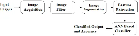
2. METHODOLOGY

The approach consists in the main of 2 half: the image process half and also the classification and testing part. Many approaches that may be helpful for the image process half exist. The main target here is on segmentation that has been shown to be terribly helpful in issues like the one at hand. Within the segmentation stage K-mean bunch is employed to extract the hemorrhage region from the image. Within the following step, discriminative options of the region of interest (ROI) are extracted. Finally, within the classification stage the image is assessed supported the computed options of the ROI. MATLAB code is written to hold out the image process and segmentation moreover because the options extraction elements, whereas the wood hen tool was used for the classification and testing elements.

Images of the patient are non-inheritable and keep at a standard place. Some pictures are of traditional patients that aren't affected by any wellness and rest is abnormal brain pictures. The pictures that are already categorized as cancerous and non-cancerous are used for reference and are used for checking the potency of planned system. Pictures are scanned and checked by radiologists whereas rummaging magnetic resonance imaging. The initial step when assortment of mister image is to convert them in gray level and playing preprocessing.

At first image pre-processing is finished through bar chart deed. Tumor features a dark look within the image therefore bar chart deed is employed to create the perimeters visible. Moot information is gift within the medical pictures. Noise and inconsistencies may be removed and quality of image and improvement of options also are consummated through image pre-processing techniques.

A method within which bar chart of a picture is obtained and its distinction is adjusted is termed as bar chart deed. Some pictures are having backgrounds and foregrounds with completely different intensities; in these cases this deed technique may be applied. It’s additionally referred to as spatial domain improvement technique. [2].

© 2017, IRJET | Impact Factor value: 5.181 | ISO 9001:2008 Certified Journal

| Page 830

Black and white colors are assigned counting on component worth and a binary image is obtained. The process can be described by following equation:

(1)

Each pixel’s intensity value is compared with the threshold value and all the pixels having lesser value than the threshold are kept only and other pixels are removed. Every comparison is done starting from first row and first column. Given image contain salt and pepper noise which is removed in enhancement stage. The image shown in figure 2 contains the noise and in the subsequent image noise being removed and better appearance is achieved. This pre-processing step make the segmentation process more effective as the better contrast and improvement can be easily observed in the two images. The threshold value is represented by T.

Fig – 1: Research Methodology of the Proposed System

3.

IMAGE DENOISING

3.1 Median Filter

The median filter could be in style nonlinear digital filtering technique, usually accustomed take away noise. Such noise reduction could be a typical pre-processing step to boost the results of later process (for example, edge detection on associate degree image). Median filtering is incredibly wide employed in digital image process as a result of below sure conditions; it preserves edges whereas removing noise [24]. Typically called a rank filter, this abstraction filter suppresses isolated noise by substitution every pixel’s intensity by the median of the intensities of the pixels in its neighborhood. It’s wide employed in de-noising and image smoothing applications. Median filters exhibit edge-preserving characteristics (cf. linear strategies like average filtering tends to blur edges), that is incredibly fascinating for several image process applications as edges contain necessary data for segmenting, labelling and protective detail in pictures. This filter may be represented by Eq (2). (2) Where 𝑤𝐹 = 𝑤 𝑥𝑤 Filter window with pixel (𝑢,𝑣) as its middle

3.2 Gaussian Filter

Gaussian filter could be a filter whose impulse response is Gaussian operate [25]. Gaussian filters square measure designed to offer no overshoot to a step operate input whereas minimizing the increase and fall time. This behavior is closely connected to the actual fact that the Gaussian filter

has the minimum attainable cluster delay. Mathematically, a Gaussian filter modifies the signal by convolution with a Gaussian function; this demodulation is additionally referred to as the Weierstrass transform. Smoothing is usually undertaken mistreatment linear filters like the Gaussian operate (the kernel relies on the conventional distribution curve), that tends to provide smart ends up in reducing the influence of noise with relation to the image. The 1D and 2D Gaussian distributions with standard deviation for a data point (x) and pixel (x,y), are given by Eq (3) and Eq (4), respectively [26].

(3)

(4) The kernel might be extended to more dimensions likewise. For a picture, the 2nd statistical distribution is employed to produce a point-spread; i.e. blurring over neighboring pixels. This is often enforced on each picture element within the image exploitation the convolution operation. The degree of blurring is controlled by the letter of the alphabet or blurring constant, likewise because the size of the kernel used (squares with associate odd variety of pixels; e.g. 3×3, 5×5 pixels, in order that the picture element being acted upon is within the middle). The process is accelerated by implementing the filtering within the frequency instead of spatial domain, particularly for the slower convolution operation (which is enforced because the quicker multiplication operation within the frequency domain).

3.3 Wiener Filter

Wiener filters are a category of optimum linear filters that involve linear estimation of a desired signal sequence from another connected sequence. It’s not reconciling filter. The wiener filter’s main purpose is to scale back the number of noise gift in a picture by comparison with estimation of the required quiet image. The Wiener filter may additionally be used for smoothing. This filter is that the mean squares error-optimal stationary linear filter for pictures degraded by additive noise and blurring. It’s sometimes applied within the frequency domain (by taking the Fourier transform) [26], owing to linear motion or unfocussed optics Wiener filter is that the most significant technique for removal of blur in pictures. From a symbol process stand. Every component in an exceedingly digital illustration of the photograph ought to represent the intensity of one stationary purpose ahead of the camera. Sadly, if the shutter speed is just too slow and therefore the camera is in motion, a given component is amalgram of intensities from points on the road of the camera's motion.

© 2017, IRJET | Impact Factor value: 5.181 | ISO 9001:2008 Certified Journal

| Page 831

spectral properties of the first signal and therefore the noise, and one seeks the LTI filter whose output would return as near the first signal as doable [27]. Wiener filters are characterized by the following:

1. Assumption: signal and (additive) noise are stationary linear random processes with known spectral characteristics.

2. Requirement: the filter must be physically realizable, i.e. causal (this requirement can be dropped, resulting in a non-causal solution).

3. Performance criteria: minimum mean-square error. Wiener Filter in the Fourier Domain as in Eq (5).

(5)

Where (𝑢,𝑣) = Fourier transform of the point spread function 𝑃(𝑢,𝑣) = Power spectrum of the signal process, obtained by taking the Fourier transform of the signal autocorrelation 𝑃(𝑢,𝑣) = Power spectrum of the noise process, obtained by taking the Fourier transform of the noise autocorrelation It should be noted that there are some known limitations to Wiener filters. They are able to suppress frequency components that have been degraded by noise but do not reconstruct them. Wiener filters are also unable to undo blurring caused by band limiting of (𝑢,𝑣), which is a phenomenon in real-world imaging systems. 4.FEATURE EXTRACTION: GREY LEVEL CO-OCCURRENCE MATRICES (GLCM) The textural choices supported gray-tone abstraction dependencies have a general connection in image classification. The three elementary pattern components utilized in human interpretation of images square measure spectral, textural and discourse choices. Spectral choices describe the everyday tonal variations in varied bands of the visible and/or infrared portion of a spectrum. Textural choices contain information concerning the abstraction distribution of tonal variations at intervals a band. The fourteen textural decisions contain data regarding image texture characteristics like homogeneity, gray-tone linear dependencies, contrast, choice and nature of boundaries gift and therefore the quality of the image. Discourse decisions contain data derived from blocks of pictorial information encompassing the realm being analyzed. Haralicket all initial introduced the utilization of co-occurrence prospects victimization GLCM for extracting varied texture decisions. GLCM is additionally referred to as grey level Dependency Matrix. It’s printed as “A two dimensional chart of gray levels for an attempt of pixels that square measure separated by a tough and quick abstraction relationship.” GLCM of an image is computed using a displacement vector d, printed by its radius δ and orientation θ. ponder a 4x4 image pictured by figure 1a with four gray-tone values zero through 3. A generalized GLCM for that image is shown in table1 where stands for style of times gray eight tones i and j neighbors satisfying the condition declared by displacement vector d. Texture options from GLCM variety of texture options is also extracted from the GLCM [20]. We have a tendency to use the subsequent notation: Here G stands for variety of grey levels taken. µ is parameter stands for the normalization of P. , , and are the parameters and customary deviations of and . (i) is that the ith entry within the marginal-probability matrix obtained by summing the rows of [21] H (6)

(7)

(8)

(9)

(10) (11) and (12)

for k=0,1,…..2(G-1). (13)

for k=0,1,…..2(G-1). Homogeneity, Angular Second Moment (ASM)[22] (14)

Angular Second Moment is the measurement of homogeneity of an image. A homogeneous picture contained some gray levels, provide a grey level co-occurrence matrix with a relatively larger but few values of P(i, j). Thus larger values will be obtained after summing of squares. Contrast [22] (15) The contrast measurement or variation in image will contribute from P(i, j) away from the diagonal, i.e. . Local Homogeneity, Inverse Difference Moment (IDM) [22]: (16)

Inverse Difference Moment is a parameter that is affected by the homogeneity term of the image. Due to weighting factor Inverse Difference Moment will lead little contributions from nonhomogeneous zone ( ). Energy [23] (17)

Entropy [22] (18) Nonhomogeneous images have little first order entropy, while a homogeneous picture has larger entropy. Auto Correlation[23]: (19)

© 2017, IRJET | Impact Factor value: 5.181 | ISO 9001:2008 Certified Journal

| Page 832

(20)

Correlation is the measurement of gray level linear dependence between the pixels at the specified positions relative to each other.

Sum of Squares, Variance[22]

(21) This parameter is most effective element which provide relatively high weights on the image elements that is different from the average value of H(i, j).

Sum Average[22]

(22)

5. SVM BASED CLASSIFICATION

SVM is a classification algorithm for high-dimensional data analysis which is proposed by Vapnik to solve the classification problems of two issues [28]. SVM has been widely used in the fields of medical image processing, text analysis, image retrieval and so on. SVM is based on the principle that the data in the original input space can be linear separable in a higher-dimensional feature space after a certain mapping. The feature space after mapping is a complete Hilbert space, in which the inner product of data can be calculated as the equivalent function value of the input vectors by introducing the corresponding kernel function. The inner product is the measurement of the distance, which can be expressed as the degree of similarity between two vectors in a certain extent. In general, the closer the distance between two vectors is, the higher the similarity of them is. Due to the kernel function, the computation of distance in the feature space is transformed to the input space without the need to solve the mapping of spatial transformation, therefore, it reduces the computational difficulty to a certain extent.

SVM has many extensions, such as one-classification SVM, in which all the interested data will be considered as one class and all the other data as the other class. In the classification, the training is only fulfilled on the data of the first class. This is a simple application of two-class SVM classification [29]. Another important application of SVM is the multi-kernel SVM [30-31]. It is especially suitable for dealing with high-dimensional data of different sources and different types. The classification algorithm does not use a uniform kernel function in order to be able to dig the implicit information in the data and to take full use of the characteristics in the data. In general, the multi-kernel SVM has two typical forms: 1. For different types of input data from different sources, use different kernel functions or different parameters with a same kernel function to design different classifiers for each input respectively, select the optimal parameters to classify each input one by one to obtain the optimal results. The final

result is the integration of all the optimal results of the input data;

2. First, some strategy is adopted to fuse all the input data, and then use different kernel functions or different parameters of a same kernel function to carry out the classification; finally using the selected fusion strategy to obtain the integrated results.

The two forms of multi-kernel SVM have very different characteristics. The former takes full use of the properties of their own in different types of data, which are independent. The use of different kernel functions can mine a variety of important and implied characteristics of data and the ultimate classification result is the integration of all the optimal results. The latter fuses the data first to use the implicit information, characteristics or relationship in various data, although different kernel functions are applied to all the parts of the data. The more important point in this processing mode is to use the correlation and mutual influence of data to achieve the classification. In addition to adapt to multiple types of input data, multi-kernel SVM can also extended to the multi-class classification problem. At present, the multi-class classification problems on brain tissues’ detection mainly depends on the fuzzy theory or the probability models, both of which are not very accurate in general. Some algorithms can just segment edema and normal tissues separately, which indicates the lack of ability to deal with brain tumors.

There is no specific multi-class classification algorithm in traditional SVM. The existing multi-class classification strategies are the simple expansions of two-class classification algorithms, such as a commonly used one versus all strategy, in which it is necessary to construct a two-class classifier for each classification of different data. The interested data will be considered as one class and all of the other data as the other class. Each class has its special classifier to make the margin between this class of samples and the other samples the largest. Then the multi-class classification can be achieved by determine each category one by one.

6. RESULTS & DISCUSSION

In this project, method consists of three stages:

Step 1. Preprocessing (including feature extraction and feature reduction);

Step 2. Training the kernel SVM;

Step 3. Submit new MRI brains to the trained kernel SVM, and output the prediction.

© 2017, IRJET | Impact Factor value: 5.181 | ISO 9001:2008 Certified Journal

| Page 833

or nerves. Database of benign MRI images are shown in fig - 2.

Fig – 2: Benign MRI Images

Malignant tumorsare cancerous and are made up of cells that grow out of control. Cells in these tumors can invade nearby tissues and spread to other parts of the body. Sometimes cells move away from the original (primary) cancer site and spread to other organs and bones where they can continue to grow and form another tumor at that site. This is known as metastasis or secondary cancer. Metastases keep the name of the original cancer location. eg. pancreatic cancer that has spread to the liver is still called pancreatic cancer.

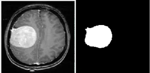
Database of malignant MRI images are shown in fig - 3.

Fig – 3: Malignant MRI Images [32]

Testing of MRI image is done using MATLAB software. In second step segmentation of selected image is done by clicking on segmented image tab. In third step classification is done suing KSVM technique and result is shown in tumer type box.

© 2017, IRJET | Impact Factor value: 5.181 | ISO 9001:2008 Certified Journal

| Page 834

Fig – 4: Test 1 (a) Original MRI Image (b) Segmented Image

Original image is inserted to system and after its segmentation support vector machine start and check the features and finding matching with data base finally evaluate the type of tumor, which is Benign type tumor resulted for above image. And accuracy is also calculated, RBF accuracy is 80%, linear accuracy is 80%, polygonal accuracy is 80% and quadratic accuracy is 90%.

Another image is taken for classification as shown original MRI image in fig. 5(a) and its segmented image is shown in fig. 5(b)

Fig – 5: Test 2 (a) Original MRI Image (b) Segmented Image

This tested image is resulted malignant type tumor. And accuracy is also calculated, RBF accuracy is 80%, linear accuracy is 90%, polygonal accuracy is 80% and quadratic accuracy is 80%.

7. CONCLUSION

In this research paper an introduction to different type of MRI image classification techniques are introduced and special focus on support vector machine. And how classification accuracy can be achieved depending on the changes and other neural approaches. Neural when combined with fuzzy logic also gives an efficient classifier. The classifiers described in this thesis categorizes the image as normal and abnormal and present the location of tumour via clustering. The manual procedure that pathologist choose for diagnosis is microscopic detection which is often time consuming and causes fatigue to them, hence this proposed system is quite beneficial . But there are several forms in

which a tumour is categorized depending upon the size and location of tissues inside the brain.

REFERENCES

[1] A. K. Jain, 1989, “Fundamentals of digital image processing,” Prentice-Hall Inc., Englewood Cliffs, New Jersey. [2] J. S. Lee, 1980, “Digital image enhancement and noise filtering by use of local statistics,” IEEE Trans. on PAMI, Vol.2, No.2, pp.165- 168.

[3] S. G. Chang, B.Yu and M. Vetterli, 2000, “Spatially adaptive wavelet thresholding with context modeling for image denoising,” IEEE Trans. on Image Processing, Vol.9, No.9, pp. 1522-1531.

[4] M. K. Mihcak, I. Kozintsev, and K. Ramchandran, 1999, “Spatially Adaptive Statistical Modeling of Wavelet Image Coefficients and its Application to Denoising,” Proc. IEEE Int. Conf. Acoust., Speech, Signal Processing, Vol.6, pp. 3253– 3256.

[5] M. Sezgin, B. Sankur. Survey over Image Thresholding Techniques and Quantitative Performance Evaluation [J]. Journal of Electronic Imaging, 2004, 13 (1): 146–165. [6] Y.J. Zhang. Image Processing and Analysis [M]. Beijing: Tsinghua University Press, 1999.

[7] N. Otsu. A Threshold Selection Method from Gray-Level Histograms [J]. IEEE Transactions on System, Man and Cybernetics, 1979, 9 (1): 62-66.

[8] R.C. Gonzalez. Digital Image Processing [M]. Peking: Publishing House of Electronics Industry, 2003.

[9] M.R. Kaus, S.K. Warfield, P.M. Black, et al. Automated Segmentation of MR Images of Brain Tumors [J]. Radiology, 2001, 218: 586-591.

[10] M. Prastawa, E. Bullitt, S. Ho, et al. A Brain Tumor Segmentation Work based on Outlier Detection [J]. Medical Image Analysis, 2004, 8: 275-283.

[11] M. Prastawa, E. Bullitt, N. Moon, et al. Automatic Brain Tumor Segmentation by Subject Specific Modification of Atlas Priors [J]. Medical Image Computing, 2003, 10: 1341-1348.

[12] M.B. Cuadra, C. Pollo, A. Bardera, et al. Atlas-based Segmentation of Pathological MR Brain Images Using a Model of Lesion Growth [J]. IEEE Transactions on Medical Imaging, 2004, 10: 1301-1313.

[13] P.Y. Lau, F.C.T. Voon, and S. Ozawa. The Detection and Visualization of Brain Tumors on T2-weighted MRI Images Using Multiparameter Feature Blocks [C]. 27th IEEE Annual Conference of the Engineering in Medicine and Biology (EMBS), 2005: 5104-5107.

[14] R.A. Lerski, K. Straughan, L.R. Schad, et al. MR Image Texture Analysis: An Approach to Tissue Characterization [J]. Magnetic Resonance Imaging, 1993, 11: 873-887.

© 2017, IRJET | Impact Factor value: 5.181 | ISO 9001:2008 Certified Journal

| Page 835

Pattern Recognition and Applications (ICSPPRA), 2001: 132-137.

[16] R. Nezafat and H. Soltanian-Zadeh. Multiwavelet-based Feature Extraction for MRI Segmentation [C]. Processing of SPIE Wavelet Applications in Signal and Imaging Processing, 1998, 3458: 182-191.

[17] K.M. Ifterkharuddin, M.A. Islam, J. Shaik, et al. Automatic Brain Tumor Detection in MRI: Methodology and Statistical Validation [C]. Proceedings of Medical Imaging, 2005, 5747: 2012-2022.

[18] S. Herlidow-Meme, J.M. Constans, B. Carsin, et al. MRI Texture Analysis on Texture Test Objects, Normal Brain and Intracranial Tumors [J]. Magnetic Resonance Imaging, 2001, 21: 989-993.

[19] Z.Q. Bian and X.G. Zhang. Pattern Recognition [M]. Beijing: Tsinghua University Press, 2000.

[20] R. M. Haralick, K. Shanmugam and I. Dinstein “Textural features for Image Classification”, IEEE Transactions on Systems, Man and Cybernetics, Vol.3, pp. 610-621, November 1973.

[21] JC-M. Wu, and Y-C. Chen, “Statistical Feature Matrix for Texture Analysis”, Computer Vision, Graphics, and Image Processing; Graphical Models and Image Processing, Vol. 54, pp. 407-419, 1992.

[22] M.M. Trivedi, R.M. Haralick, R.W. Conners, and S. Goh, ”Object Detection based on Gray Level Co-ocurrence”, Computer Vision, Graphics, and Image Processing, Vol. 28, pp. 199-219, 1984.

[23] Sushila Shidnal, “A texture feature extraction of crop field images using GLCM approach”, IJSEAT, Vol 2, Issue 12, December – 2014.

[24] H. Raymond Chan, Chung-Wa Ho, and M. Nikolova, “Salt-and-Pepper noise removal by median-type noise detectors and detail-preserving regularization”. IEEE Trans Image Process 2005; 14: 1479-1485.

[25] P. Hsiao1, S. Chou, and F. Huang, “Generic 2-D Gaussian Smoothing Filter for Noisy Image Processing”. National University of Kaohsiung, Kaohsiung, Taiwan, 2007. [26] S. Kumar, P. Kumar, M. Gupta and A. K. Nagawat, “Performance Comparison of Median and Wiener Filter in Image De-noising,” International Journal of Computer Applications 12(4):27–31, December 2010.

[27] Kazubek, “Wavelet domain image de-noising by thresholding and Wiener filtering”. M. Signal Processing Letters IEEE, Volume: 10, Issue: 11, Nov. 2003 265 Vol.3. [28] V. Vapnik. The Nature of Statistical Learning Theory [M]. London: Springer, 1995.

[29] J. Zhou, K.L. Chan, V.F.H. Chong, et al. Extraction of Brain Tumor from MR Images Using One-Class Support Vector Machine [C.] 27th Annual International Conference on Engineering Medicine and Biology Society (EMBS), 2005: 6411-6414.

[30] Z. Wang, S.C. Chen and T.K. Sun. MultiK-MHKS: A Novel Multiple Kernel Learning Algorithm [J]. IEEE Transactions on