http://dx.doi.org/10.4236/jsip.2015.62008
Under What Condition Do We Get Improved
Equalization Performance in the Residual ISI
with Non-Biased Input Signals Compared
with the Biased Version
Monika Pinchas
Department of Electrical and Electronic Engineering, Ariel University, Ariel, Israel Email: [email protected]
Received 27 January 2015; accepted 1 April 2015; published 2 April 2015 Copyright © 2015 by author and Scientific Research Publishing Inc.
This work is licensed under the Creative Commons Attribution International License (CC BY).
http://creativecommons.org/licenses/by/4.0/
Abstract
Recently, closed-form approximated expressions were obtained for the residual Inter Symbol In-terference (ISI) obtained by blind adaptive equalizers for the biased as well as for the non-biased input case in a noisy environment. But, up to now it is unclear under what condition improved equalization performance is obtained in the residual ISI point of view with the non-biased case compared with the biased version. In this paper, we present for the real and two independent qu-adrature carrier case a closed-form approximated expression for the difference in the residual ISI obtained by blind adaptive equalizers with biased input signals compared with the non-biased case. Based on this expression, we show under what condition improved equalization performance is obtained from the residual ISI point of view for the non-biased case compared with the biased version.
Keywords
Residual ISI, Blind Equalization, Blind Deconvolution
1. Introduction
We consider a blind deconvolution problem in which we observe the output of an unknown, possibly nonmini- mum phase, linear system from which we want to recover its input using an adjustable linear filter (equalizer)
[1]-[5]. The problem of blind deconvolution arises comprehensively in various applications such as digital com-
image restoration [1] [2] [6]. The above mentioned possibly nonminimum phase, linear system may be considered for instance as a channel in the communication area. According to [3] [7] [8], the channel is not ideal due to reflections and delays caused by the physical environment such as ground, buildings and cables. Those reflections and delays cause distortion of the received signal which is referred as ISI [3] [9]. Thus, a blind adaptive equalizer may be used to remove the unwanted ISI of the system to produce the source signal [10]-[14]. According to [1]-
[3] [15], the equalization performance depends on the nature of the chosen equalizer (on the memoryless non-
linearity situated at the output of the equalizer’s filter), on the channel characteristics, on the added noise, on the step-size parameter used in the adaptation process, on the equalizer’s tap length and on the input signal statistics. Fast convergence speed and reaching a residual ISI where the eye diagram is considered to be open (for the communication case) are the main requirements from a blind equalizer [1]-[3] [15]. Fast convergence speed may be obtained by increasing the step-size parameter [1]-[3] [15]. But, increasing the step-size parameter may lead to a higher residual ISI which may not meet any more the system’s requirements [1]-[3] [15]. Up to recently, we used time consuming simulation for performance assessment. Recently, closed-form approximated expressions were obtained for the residual ISI valid for the noiseless and unbiased input signal case [15], noisy and unbiased input signal case [1], noisy and unbiased input signal case but where the gain between the equalized output and input signal is equal or less than one [16] and for the noisy and biased input signal case [3]. But, up to now it is unclear under what condition improved equalization performance is obtained in the residual ISI point of view with the non-biased case compared with the biased version.
In this paper, we derive for the real and two independent quadrature carrier case a closed-form approximated expression for the difference in the residual ISI obtained by blind adaptive equalizers with biased input signals compared with the non-biased case. This expression depends on the step-size parameter, equalizer’s tap length, input signal statistics, channel power and signal to noise ratio (SNR). In addition, this expression is valid for blind adaptive equalizers where the error fed into the adaptive mechanism, which updates the equalizer’s taps, can be expressed as a polynomial function of order three of the equalized output and where the gain between the input and equalized output signal is equal to one as is in the case of Godard’s algorithm [17]. Based on this new derived expression we show under what condition improved equalization performance is obtained from the resi- dual ISI point of view for the non-biased case compared with the biased version.
The paper is organized as follows. After having described the system under consideration in Section II, the condition for which improved equalization performance is obtained from the residual ISI point of view for the non-biased case compared with the biased version is introduced in Section III. In Section IV simulation results are presented and the conclusion is given in Section V.
2. System Description
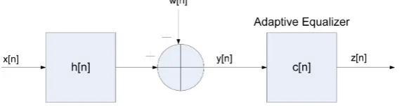
The system under consideration is the same system as shown in [1]-[3] [15] and [16]. Thus, we recall from [3]
the block diagram of the system illustrated in Figure 1. We adapt in the following most of the assumptions made in [3]:
1) The input sequence x n
[ ]
represents a two independent biased or unbiased quadrature carriers case constellation input where x nr[ ]
and x ni[ ]
are the real and imaginary parts of x n[ ]
respectively.2) The mean of the input sequence x n
[ ]
is E x n[ ]
, where E[ ]
⋅ is the expectation operator and[ ] [ ]
[ ]
x n =x n E x n−
.
3) E x n r
[ ]
=E x n i[ ]
.4) The unknown channel h n
[ ]
is modeled as a non-minimum phase FIR filter, which has zeros far from the unit circle.5) c n
[ ]
is a tap-delay line.6) The noise w n
[ ]
is an added Gaussian white noise with zero mean and consists of w n[ ]
=w nr[ ]
+ jw ni[ ]
where w nr[ ]
and w ni[ ]
are the real and imaginary parts of w n[ ]
respectively as well as w nr[ ]
and[ ]
i
w n are independent. Both w nr
[ ]
and w ni[ ]
have zero mean and their variances are denoted as:[ ]
2 2
r
w E w nr
σ = , 2 2
[ ]
i
w E w ni
Figure 1. Block diagram of a baseband communication system. 7) The variance of w n
[ ]
is denoted as[ ] [ ]
* 2w
E w n w n = σ where 2 2 2 2 2
i r
w w w
σ = σ = σ and
( )
⋅* is the conjugate operation on( )
⋅ .The transmitted sequence x n
[ ]
is sent through the channel h n[ ]
and is interfered with noise w n[ ]
. Therefore, the equalizer’s input sequence y n[ ]
may be written as:[ ] [ ] [ ] [ ]
y n =x n h n w n∗ + (1) where “∗” denotes the convolution operation. The equalizer’s output sequence may be written as:
[ ] [ ] [ ] [ ] [ ] [ ]
z n =y n c n∗ =x n +p n w n+ (2) where p[n] is the convolutional noise that arises due to the use of non-ideal equalizer’s coefficients (blind equalization) instead of the ideal set and w n
[ ]
=w n c n[ ] [ ]
∗ . The equalizer’s update mechanism is defined by:[
1] [ ]
F n[ ] [ ]
[ ]
c n c n y n
z n
µ∂ ∗
+ = −
∂ (3) where µ is the equalizer’s step-size, c n
[
+1]
and c n[ ]
are the next and current state of the equalizer's vector respectively, y n[ ]
=(
y n[ ]
y n N[
− +1]
)
T, N is the equalizer’s tap length and z n[ ] [ ]
=z n E z n− [ ]
. The operator( )
T denotes for transpose of the function () and the real part of F n[ ]
[ ]
z n
∂
∂ is a polynomial function of order three of z n
[ ]
. In this paper, the ISI is used as a measure of equalization performance and is defined by:2 2
max 2 max m
m s s
ISI
s − =
∑
(4)
where smax is the component of s, given by s c n h n=
[ ] [ ]
∗ , having the maximal absolute value. According to [3], the residual ISI expressed in dB units may be written for biased input signals as:( )
(
[ ]
2)
10 10
10log 2 10log
dB p
ISI = m − E x n (5) where
( )
⋅ is the absolute value of( )
⋅ and mp is defined by:1 1
1 1 1 1
1 1
1 2
1 2
1 2
1 2
for 0 and 0
min ,
or for 0
max ,
p p
p p
p p
p p
m m
m m
p
m m
m m
p
Sol Sol
m Sol Sol
Sol Sol
m Sol Sol
> >
=
⋅ <
=
(6)
1
1
2
1 1 1 1
1
1 2
1 1 1 1
2 1 4 2 4 2 p p m m
B B A C B
Sol
A
B B A C B
Sol A − + − = − − − = (7) where
(
)
(
)
(
)
2 2 2 2 2
1 3 3 12 1 3 12 1 12
2 2 2
3 12 3 3 12 12
45 18 6 9 2
2 3 45 18 9
r r r
r
x x x
w
A B a a a a a a a a
a a B a a a a
σ σ σ
σ = + + + + − + + + + (8)
( )
( )
(
( )
)
(
)
2 22 2 2 2 2 2 4 2 4
1 3 12 12 1 3 1 12 1 3 3 12
4 2 2 2 2 2 4
12 1 3 12 3 3 12 12
2 2 2 2 2
3 3 12 1 3 12
12 6 12 4 15 2
2 3 45 18 9
90 36 12 18
r r r r
r r r
r r r
x x x x r r
r x x w
x x
x
x
B B a a a a a a a a E x a E x a a
E x a a a a B a a a a
B a a a a a a
σ σ σ σ
σ σ σ
σ σ σ
= + + + + + + + − + + + + + + + + +
(
)
(
)
21 12 12 3
4a a 2a 6a σwr
+ − − (9)
( )
(
)
(
)
(
)
22 2 2 4 2 4 2 2 4 6 2
1 1 12 1 3 12 12 1 3 3
2 2 6 2 2 2 2 2 4
3 3 12 12 3 3 12 1 3 12 1 12
2 2 2
1 1 3 1 12
2 2 2
15 6 3 45 18 6 9 2
12 4 15
r r r r
r r r r r
r r
x x r x r x r r
w x x x w
x x
C a a a E x a a E x a E x a a E x a
a a a a a a a a a a a a
a a a a a
σ σ σ σ
σ σ σ σ σ
σ σ = + + + + + + + + + + + + + + + + +
( )
(
( )
)
22 4 2
3 3 12
2
4 2 4 2 2 2
3 12 12 12
12
2 6
r
r r
r x
r r x w
a E x a a
a a E x a E x a
σ σ σ + + + + (10)
[ ]
[ ]
2 2 2 1 0 0.5 r w R kE x n
SNR h k
σ − =
∑
(11)
[ ]
(
)
[ ]
[ ]
2 1 2 2 2 0 R x kE x n
B N E x n h k N
SNR
µ σ − µ
= +
∑
+ (12)
R is the channel length, a1, a12, a3 are properties of the chosen equalizer and found by:
[ ]
[ ]
(
1( )
r 3( )
r 3 12( )( )
r i 2)
F n
Re a z a z a z z
z n
∂
= + +
∂
(13)
where Re
( )
⋅ is the real part of( )
⋅ and zr, zi are the real and imaginary parts of z n[ ]
, σx2r is the varianceof x nr
[ ]
(x nr[ ]
is the real part of x n[ ]
), σx2 is the variance of x n[ ]
and SNR is given by:[ ]
2 2 wE x n
3. Condition for Improved Equalization Performance
In this section, we first derive a closed-form approximated expression for the difference in the residual ISI obtained by blind adaptive equalizers with biased input signals compared to the non-biased case. Then, based on this new derived expression, we derive the condition for which improved equalization performance is obtained from the residual ISI point of view for the non-biased input case compared to the biased version. In the following we denote ISIdB, A1, B1, B and SNR for the non-biased case (by substituting E x n
[ ]
= 0 into (5), (8), (9), (12) and (14)) as ISInb, A1nb, B1nb, Bnb and SNRnb respectively. In addition, for the biasedcase, we denote (5), (8), (9), (12) and (14) as ISIb, A1b, B1b, Bb and SNRb respectively. To facilitate reading,
we denote E x n
[ ]
as m. Theorem: 10 2 2 1 10 2 2 1 1 10log 1 1 1 10log 1 1 b nb nb nb nb x nb x b B ISI ISI m bb B b B ISI m bb B σ σ + = + + + ⇓ + ∆ = + + (15)where ∆ISI is the closed-form approximated expression for the difference in the residual ISI obtained by blind adaptive equalizers with biased input signals compared to the non-biased case and
[ ]
1 2 2 0 R k b µN m − h k=
=
∑
(16)(
)
( )
( )
4 2
2 2
2 2 2 2 2 2
3 12 12 1 3 1 12 1
4 2 4 4 2
3 3 12 12
2 2
3 3 12 12
2 2 2 2 2
3 3 12 1 3 12 1 12
12 6 12 4
15 2
45 18 9
90 36 12 18 4
r r
r r r r
r r r
w w
x x x x
r r r
x x x
bb b a r q
a a a a a a a a a
E x a E x a a E x a
r a a a a
q a a a a a a a a
σ σ
σ σ σ σ
σ σ σ
= + + = + + + + + + + = + + = + + + +
(17)
Proof:
Based on (14) we have:
2 2 2
2 2
2 2 1 2 1 2
x x
b nb
w w x x
m m m
SNR σ σ SNR
σ σ σ σ
+ = = + = + (18)
With the help of (11) and (18) we may write:
(
)
[ ]
[ ]
[ ]
[ ]
2
2 2 2
2
1 2 2 2 1
2 2 0 0 2 2 2
1 2 1 2
0 0
1 1 1
2 2 1 1 2 r r r x x w R R x b nb k k x x x
w R R
nb nb
k k
m m
m
SNR h k SNR h k
SNR h k SNR h k
From (19) we may conclude that C1 (10) has the same value for the biased and non-biased input case. Next, we wish to find the relationship between Bb and Bnb and between B1b and B1nb. For that purpose we use
(12) and (18) to obtain:
(
)
[ ]
(
)
[ ]
2 2
2
2 2 2
1 2 1 2
2 2 2 2 2 0 0 2 1 1 1 x
R x R x
b x x
k b x k
nb x m N
N m m
B N m h k N h k
SNR m
SNR
µ σ
µ σ σ
µ σ µ σ
σ σ − − = = + + = + + = + + +
∑
∑
(20)From (20) we have:
[ ]
2 1 2
2 2
2 0
1 R x
b x
k nb
x
m N
B N h k
SNR µ σ µ σ σ − = = + +
∑
(21)Next by substituting m=0 into (12) and using (18), we may write (21) as:
[ ]
1 2
2
0 R
b nb nb
k
B B µN m − h k B b
=
= +
∑
= + (22)where
[ ]
21 2 2 0 R x nb x k nb N
B N h k
SNR
µ σ µ σ −
=
=
∑
+ (23)
and b is given in (16). Based on (22) we may write:
1 b nb nb b B B B = +
(24)
Next we turn to find the relationship between B1b and B1nb. From (9) we may write:
(
)
4 2
1b b b wr b wr
B =B a s B r− + σ + B q d− σ (25) where a, r and q are given in (17) and
(
2 2)
1 3 12
12 3
2 3
2 6
r r
x x
s a a a
d a a
σ σ
= + +
= +
(26)
From (25) and (24) we may have:
(
)
(
)
4 2 2
1
4 2 2
1
b r r r
r r r
b w w w
nb w w w
nb
B B a r q d s
b
B a r q d s
B
σ σ σ
σ σ σ
= + + − − = + + + − − (27)
which can be also written as:
(
4 2)
1 1 1 1
1 1
b nb r r nb nb
nb
w w bb
B B b a r q B bb B
B
σ σ
= + + + = + = +
(28)
where bb is given in (17) and B1nb is obtained by substituting m=0 into (9):
(
4 2)
21nb nb wr wr wr
B =B a r+ σ +qσ −dσ −s (29) The solution for mp given in (6) is acually based on the following second order equation with respect to p
m [15]:
2
1 p 1 p 1 0
According to [15], mp may be very small in the convergence state so that the part of A m1 2p may be neglectable compared to B m1 p+BC1. If this is the case then the solution for mp is:
1
1
p BC
m B
= − (31) Simulation results carried out in [15] have shown that better accuracy is obtained when using (6) over (31) for the non-biased case which is not surprising. But, the difference in the accuracy is not so high making the solution for mp given in (31) acceptable. In the following we denote mp as mpb and mpnb for the biased
and non-biased input case respectivaly. By using (31), (28) and (24) we may have:
1 1
1 1
1 1 1
1
1 1 1
1 1 1 1
1 1 1
b nb
b nb
nb
nb nb nb
nb nb
nb nb nb nb
b nb
p p
b
b b b b
B C B C
B B B B
B C B C
m m
B B bb B bb bb
B
B B B
+ + + + = − = − = − = − = + + + (32) where 1 1 nb nb nb
p B C
m
B
= − (33) Next, by using (5) we may have:
(
)
(
)
(
)
(
)
( )
2 2 10 10 2 210 10 2
2 2
10 10 10 2
10log 2 10log
10log 2 10log 1
10log 2 10log 10log 1
b
b
b
b p x
p x
x
p x
x
ISI m m
m m m m σ σ σ σ σ = − + = − + = − − + (34)
Now we substitute (32) into (34) and obtain:
( )
(
)
( )
(
)
2 2
10 10 10 2
1
2 2
10 10 10 10 2
1
10 10
1
10log 2 10log 10log 1
1
1
10log 2 10log 10log 10log 1
1
10log 2 10log
nb nb nb nb nb nb
b p x
x nb p x x p b B m ISI m bb B b m B m bb B m σ σ σ σ σ + = − − + + + = + − − + + = −
( )
2 210 10 2
1
2
10 10 2 10 2
2 1
1 1
10log 10log 1
1
1 1
10log 10log 1 10log
1 1 1
nb nb nb nb x x nb nb nb nb x x b m B bb B b b m B B
ISI bb ISI
m bb B B σ σ σ + + − + + + + = + − + = + + + +
where
(
)
( )
210 10
10log 2 nb 10log
nb p x
ISI = m − σ (36)
This completes our proof. b
ISI as well as ISInb (15) hold negative values. Perfect equalization performance in the residual ISI point of view is achieved for the biased case if ISIb→ −∞. In addition, perfect equalization performance in the residual ISI point of view is achieved for the non-biased case if ISInb→ −∞. Thus, if ∆ISI (15) is positive
(
∆ISI>0)
it implies that improved equalization performance is obtained in the residual ISI point of view for the non-biased case compared with the biased version. In other words, according to (15), if2
2 1
1 1 1
nb
nb x
m
b bb
B B σ
+ > + +
(37)
then improved equalization performance is obtained from the residual ISI point of view for the non-biased input
case compared to the biased version. In the following we will show the relationship between nb b B and
2
2 x m
σ .
By using (16) and (23) we have:
[ ]
[ ]
[ ]
[ ]
1 2 1 2
2
2 2
0 0
2 2 1 2
1 2 2
2
0 0
1
R R
k k
R R
nb x x x
x
k nb
k nb
N m h k m h k m
b
B N h k N h k
SNR SNR
µ
µ σ σ σ
µ σ
− −
= =
− −
= =
= = ≤
+ +
∑
∑
∑
∑
(38)
Thus, according to (38), we may conclude that if 1
0
nb
bb
B > then improved equalization performance is ob- tained from the residual ISI point of view for the biased input case compared to the non-biased version. Please note that (37) depends on the step-size parameter, equalizer’s tap length, input signal statistics, channel power, signal to noise ratio and on the properties of the chosen blind equalizer via a1, a12 and a3 from (13).
4. Simulation
In this section, ∆ISI (15) was tested via simulation by using Godard’s algorithm [17]. Please note that if 0
ISI
∆ > then improved equalization performance is obtained in the residual ISI point of view for the non- biased input case compared with the biased version. The equalizer’s taps for Godard’s algorithm [17] were updated according to:
[
]
[ ]
[ ]
[ ]
[ ]
[ ]
[ ]
[ ]
(
[ ]
[ ]
)
[
]
4 2
2 1
m m G
E x n E x n
c n c n z n E x n z n E x n y n m
E x n E x n
µ ∗
−
+ = − − − − −
−
(39)
where, µG is the step-size. The values for a1, a12 and a3 corresponding to Godard’s [17] algorithm are defined as a1G, a12G and a3G respectively and are given by:
[ ]
[ ]
[ ]
[ ]
4
1 2 ; 12 1; 3 1
G E x n E x n G G
a a a
E x n E x n
−
= − = =
−
(40)
A biased 16QAM, a modulation using ±{1, 3} levels for in-phase and quadrature components in addition to a given bias was considered. The bias for the real and imaginary axes were the same. In our simulation we used the channel given in [18]:
(
0 for 0; 0.4 for 0; 0.84 0.4n1 for 0)
n
h = n< − n= ⋅ − n> .
Figure 2. Simulated ISI performance comparison between the biased 16QAM input case and the non-biased version using (39) for SNRb=30 dB
[ ]
. The averaged results were obtained in 100 Monte Carlo trials.13
N= and 17 106
G
µ = × −
[image:9.595.194.402.290.455.2]. The bias was set to 6 6+ j.
Figure 3. Simulated ISI performance comparison between the biased 16QAM input case and the non-biased version using (39) for SNRb=25 dB
[ ]
. The averaged results were obtained in 100 Monte Carlo trials.13
N= and 17 106
G
µ = × − . The bias was set to 6 6+ j.
Figure 4. Simulated ISI performance comparison between the biased 16QAM input case and the non-biased version using (39) for SNRb=30 dB
[ ]
. The averaged results were obtained in 100 Monte Carlo trials.13
N= and 17 106
G
[image:9.595.195.401.510.673.2]Figure 5. Simulated ISI performance comparison between the biased 16QAM input case and the non-biased version using (39) for SNRb=20 dB
[ ]
. The averaged results were obtained in 100 Monte Carlo trials.13
N= and 17 106
G
[image:10.595.163.436.301.708.2]µ = × − . The bias was set to 4 4+ j.
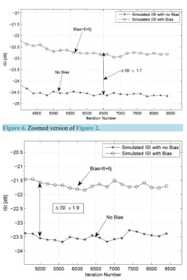
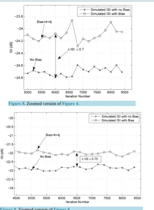
Figure 6. Zoomed version of Figure 2.
Figure 8. Zoomed version of Figure 4.
Figure 9. Zoomed version of Figure 5.
difference in the residual ISI between the biased and non-biased case is ∆ISI ≅1.7 while according to (15) we have ∆ISI ≅1.92.
According to Figure 7 the simulated difference in the residual ISI between the biased and non-biased case is 1.9
ISI
∆ ≅ while according to (15) we have ∆ISI≅2.102.
According to Figure 8the simulated difference in the residual ISI between the biased and non-biased case is 0.7
ISI
∆ ≅ while according to (15) we have ∆ISI≅0.73.
According to Figure9the simulated difference in the residual ISI between the biased and non-biased case is 0.75
ISI
∆ ≅ while according to (15) we have ∆ISI ≅0.77.
Based on Figures 6-9, the simulated results for ∆ISI and those results obtained from (15) for ∆ISI are very close. Thus, the expression for ∆ISI (15) is accurate enough for saying that if ∆ISI >0 then improved equalization performance is obtained in the residual ISI point of view for the non-biased input case compared to the biased version. Please note that according to Figures 2-5, improved equalization performance was obtained in the residual ISI point of view for the non-biased input case compared to the biased version which was also confirmed by the expression for ∆ISI (15) since ∆ISI was found to be positive for all the mentioned cases.
5. Conclusion
expression for the difference in the residual ISI obtained by blind adaptive equalizers with biased input signals compared to the non-biased case. This expression depends on the step-size parameter, equalizer’s tap length, input signal statistics, channel power, SNR and chosen equalizer via a1, a12 and a3. It is applicable for blind adaptive equalizers where the error fed into the adaptive mechanism, which updates the equalizer’s taps, can be expressed as a polynomial function of order three of the equalized output and where the gain between the input and equalized output signal is equal to one as is in the case of Godard’s algorithm. Based on this expression, we have shown under what condition improved equalization performance is obtained from the residual ISI point of view for the non-biased case compared with the biased version.
Acknowledgements
We thank the editor and the referee for their comments.
References
[1] Pinchas, M. (2010) A New Closed Approximated Formed Expression for the Achievable Residual ISI Obtained by Adaptive Blind Equalizers for the Noisy Case. IEEE International Conference on Wireless Communications, Network-ing and Information Security (WCNIS), Beijing, 25-27 June 2010, 26-30.
http://dx.doi.org/10.1109/WCINS.2010.5541879
[2] Pinchas, M. (2013) Residual ISI Obtained by Blind Adaptive Equalizers and Fractional Noise. Mathematical Problems in Engineering, 2013, 1-11. http://dx.doi.org/10.1155/2013/972174
[3] Panziel, N. and Pinchas, M. (2014) An Approximated Expression for the Residual ISI Obtained by Blind Adaptive Equalizer and Biased Input Signals. Journal of Signal and Information Processing (JSIP), 5, 155-178.
[4] Haykin, S. (1991) Blind Deconvolution. In: Haykin, S., Ed., Adaptive Filter Theory, Chapter 20, Prentice-Hall, En-glewood Cliffs.
[5] Yang, D.H., Li, G. and Zhu, Z.H. (2011) A Novel Structure for Adaptive Blind Channel Equalization. 7th International Conference on Wireless Communications, Networking and Mobile Computing (WiCOM), Wuhan, 23-25 September 2011, 1-4. http://dx.doi.org/10.1109/wicom.2011.6039953
[6] Feng, C. and Chi, C. (1999) Performance of Cumulant Based Inverse Filters for Blind Deconvolution. IEEE Transac-tion on Signal Processing, 47, 1922-1936. http://dx.doi.org/10.1109/78.771041
[7] Wen, S.-Y. and Liu, F. (2010) A Computationally Efficient Multi-Modulus Blind Equalization Algorithm. The 2nd IEEE International Conference on Information Management and Engineering (ICIME), Chengdu, 16-18 April 2010, 685-687. http://dx.doi.org/10.1109/ICIME.2010.5478261
[8] He, N. (2010) Application of Adaptive Equalizer in Digital Microwave Communication. International Conference on Electronics and Information Engineering (ICEIE), 2, 497-500. http://dx.doi.org/10.1109/ICEIE.2010.5559759
[9] Sheikh, S.A. and Fan, P.Z. (2008) New Blind Equalization Techniques Based on Improved Square Contour Algorithm.
Digital Signal Processing, 18, 680-693. http://dx.doi.org/10.1016/j.dsp.2007.09.001
[10] Sato, Y. (1975) A Method of Self-Recovering Equalization for Multilevel Amplitude Modulation. IEEE Transactions on Communications, 23, 679-682. http://dx.doi.org/10.1109/TCOM.1975.1092854
[11] Tuğcu, E., Çakır, F. and Ozen, A. (2013) A New Step Size Control Technique for Blind and Non-Blind Equalization Algorithms. Radioengineering, 22, 4-51.
[12] Liu, Z. and Ning, X.L. (2012) Comparison of Equalization Algorithms for Underwater Acoustic Channels. The 2nd In-ternational Conference on Computer Science and Network Technology, Changchun, 29-31 December 2012, 2059-2063. http://dx.doi.org/10.1109/ICCSNT.2012.6526324
[13] Vanka, R.N., Murty, S.B. and Mouli, B.C. (2014) Performance Comparison of Supervised and Unsupervised/Blind Equalization Algorithms for QAM Transmitted Constellations. 2014 International Conference on Signal Processing and Integrated Networks (SPIN), Noida, 20-21 February 2014, 316-321.
http://dx.doi.org/10.1109/SPIN.2014.6776970
[14] Qin, Q., Li, H.H. and Jiang, T.Y. (2013) A New Study on VCMA-Based Blind Equalization for Underwater Acoustic Communications. 2013 International Conference on Mechatronic Sciences, Electric Engineering and Computer (MEC), Shenyang, 20-22 December 2013, 3526-3529.
[15] Pinchas, M. (2010) A Closed Approximated Formed Expression for the Achievable Residual Intersymbol Interference Obtained by Blind Equalizers. Signal Processing, 90, 1940-1962.
http://dx.doi.org/10.1016/j.sigpro.2009.12.014
Adaptive Equalizers with Gain Equal or Less than One. Radioengineering, 23, 954.
[17] Godard, D.N. (1980) Self Recovering Equalization and Carrier Tracking in Two-Dimensional Data Communication System. IEEE Transactions on Communications, 28, 1867-1875. http://dx.doi.org/10.1109/TCOM.1980.1094608 [18] Shalvi, O. and Weinstein, E. (1990) New Criteria for Blind Deconvolution of Nonminimum Phase Systems (Channels).
![Figure 2. Simulated ISI performance comparison between the biased 16QAM input case and the non-biased version using (39) for SNR30 dB[]b =](https://thumb-us.123doks.com/thumbv2/123dok_us/8149110.801973/9.595.195.401.510.673/figure-simulated-performance-comparison-biased-biased-version-using.webp)