http://dx.doi.org/10.4236/tel.2014.49110
How to cite this paper: Lahiri, B. (2014) The Effect of Environmental Taxes on Steady-State Consumption. Theoretical Eco-nomics Letters, 4, 867-874. http://dx.doi.org/10.4236/tel.2014.49110
The Effect of Environmental Taxes on
Steady-State Consumption
Bidisha Lahiri
Department of Economics and Legal Studies, Oklahoma State University, Stillwater, USA Email: bidisha.lahiri@okstate.edu
Received 19 October 2014; revised 28 November 2014; accepted 12 December 2014
Copyright © 2014 by author and Scientific Research Publishing Inc.
This work is licensed under the Creative Commons Attribution International License (CC BY).
http://creativecommons.org/licenses/by/4.0/
Abstract
This paper examines the effects of environmental taxes on the demand and supply sides of the economy and uncovers two opposite forces on long-term production. An increase in the environ-mental tax stimulates abatement behavior as producers lower production from the same capital stock but simultaneously lower per-unit emissions increases consumers’ demand for the cleaner goods hence increasing the capital stock. Starting from a low level of environmental taxes, my model finds that initially the demand-driven positive relationship dominates while at a higher level of environmental taxes, the production lowering negative effect dominates; the transition occurs before the economy reaches the optimal tax rate.
Keywords
Environmental Tax, Steady State, Production, Emission
1. Introduction
equiv-868
alent to greater environmental wealth. For future generations, this is equivalent to the positive income effect of a high pollution tax in the long run. Grimaud and Rouge [4] assume that emissions generated during production have a negative effect on welfare. Using an endogenous growth model, they find that a carbon tax has a negative impact on short-term production and consumption but has a positive impact on long-term growth.
In a slightly different approach, Gupta and Ray Burman [5] consider the allocation of government income tax revenue across abatement expenditures and productive public expenditures. In their model, a higher share of ab-atement expenditures improve the efficiency of productive public expenditures, generating the positive effect of pollution control. Acemoglu et al. [6] consider the effect of environmental policies toward endogenous technol-ogy. When stricter environmental policies encourage technological innovation, a positive effect on production emerges.
This theoretical literature shows that a stricter environmental policy is not incompatible with a positive effect on economic production; however, in showing this result, the studies rely on strong assumptions that may appear to favor such results. In the current paper, I uncover the positive (and negative) effects of stricter environmental policies in a simple model that is not based on a priori assumptions regarding the positive effect of the policies. Instead, the model derives its results based on the observation that for consumers the trade-off between con-sumption and environmental quality is such that richer consumers prefer lower pollution while poorer consum-ers are more accepting of higher pollution if that affords them marginally more consumption. This results in a negative relationship between consumption and pollution. On the resource constraint side, a positive relationship exists between pollution and production. Introducing a change in environmental taxes in the setting of these pos-itive and negative relationships between production and pollution generates very interesting comparative statics results.
The rest of the paper is stet-up as follows. I set-up the model in Section 2 where I first elaborate the produc-tion condiproduc-tions which coupled with the resource constraint underlies the negative relaproduc-tion between environmen-tal taxes and consumption. Next I develop the demand side of the model that leads to the positive relation be-tween environmental taxes and consumption. Finally I put together the demand and supply dimensions to cha-racterize the steady state equilibrium. The effects of changes in environmental taxes are explored as comparative statics for the steady state equilibriums. Finally Section 3 concludes with a summary of the current findings and directions for future research.
2. Model
To capture the final effect of an environmental policy on long-term equilibrium (steady-state) output, I will fo-cus on how emission taxes affect both supply and demand within the economy. I introduce emissions and envi-ronmental taxes in the Neoclassical Growth Model with an endogenous savings rate developed by Ramsey [7], Cass [8] and Koopmans [9]. The price of the produced commodity Yt is normalized to one; return to capital
( )
rt , environmental taxes( )
τ
t , and the value of marginal disutility from pollution( )
Pz t, are all expressedrelative to this normalized price1.
2.1. Supply
Production
( )
Yt is a decreasing function of capital( )
Kt and emits pollution( )
Zt as a byproduct. In the absence of any abatement activity, production and emissions are given by Equation (1).( )
sy, where 1t t t t y
Y = K Z =K s ≤ . (1)
Emissions can be abated if some resources are diverted for this purpose. Following the approach popularized by Copeland and Taylor [10], the production of output and of the emission byproduct are combined into a single function using abatement technology. If
t
Y
θ is the fraction of resources spent for abatement activity in sector
t
Y, then the output level after abatement activity is:
(
)
{
1}
yt
s
t t Y
Y = K −θ . (2)
The emission level after abatement activity is:
869
(
)
11 t
t Y t
Z = −θ α′K . (3)
Here α′ is the parameter from abatement technology in the Y sector. Combining (2) and (3) by eliminat-ing
t
Y
θ between the above two production functions results in the Cobb-Douglas form of production relation-ship.
where y
s
t t t y
Y =Z Kα −α α α= ′∗s (4)
Emissions appear as an input for production; higher emissions are associated with a higher production level, implying that fewer resources are diverted for abatement of the pollution.
Suppose that the government imposes a tax τt on per-unit emissions. Profit maximizing producers will en-gage in abatement activity until the level where the marginal product of the last unit of emission equals the cost of the emission tax:
t Y Zt t
τ =α .
Using this condition to eliminate emission level Zt from production function (4) expresses production Yt as a function of capital stock and the prevailing emission tax rates as in (5).
( )
(
)
1
1 . ., ; , ,
y
s
t t t t t y t
t
Y K i e Y Y K s
α
α α
α
α α τ
τ − − − = =
(5)
I assume that emission tax revenues collected by the government are distributed back in a lump-sum manner so that they do not affect the national budget constraint. The only role of the emission tax is to ensure abatement activity by producers. Under optimal taxation where the tax level is set equal to consumers’ disutility from emissions, the optimal tax ensures that the marginal cost to producers of emission reduction equals consumers’ valuation of the marginal disutility from emissions.
2.2. Resource Constraint
Next I turn to the resource constraint of the economy that matches demand and supply. The total quantity pro-duced every period
( )
Yt is used for consumption( )
Ct and capital( )
Kt accumulation purposes.(
Kt+1−Kt)
+Ct =YtUsing (5) to represent production in the above resource constraint, I rewrite it as Equation (6).
(
)
( )
11 1
y s
t t t t
K K C K
α α α α α τ − − − + − + =
(6)
2.3. Demand
On the demand side, I assume an infinitely lived consumer whose life-time welfare is the discounted sum of every period’s welfare:
( )
0 0
ln
t t
t t t t
t t
U ρu ρ C γ Z
∞ ∞
= =
=
∑
=∑
− ⋅ . (7)In any given period, the consumer derives positive but decreasing marginal utility from consumption and dis-utility from emissions2. If
t
Z
P is the marginal valuation of pollution while the price of the produced commodity is normalized to 1 as mentioned earlier, then Equation (8) shows that although the marginal disutility of emis-sions is assumed to be constant, pollution disutility is valued more strongly as economies get richer3.
2Copeland and Taylor (1997), “A Simple Model of Trade, Capital Mobility and the Environment,” NBER Working Paper 5898. 3As the valuation of pollution disutility becomes larger as
t t
870
, or 1
t
t
Z t t
Z t
t t
P u Z
P C
u C
γ
−∂ ∂
= =
∂ ∂ (8)
Equation (9) is the Euler equation that embodies the first-order condition for maximizing intertemporal wel-fare (7) with respect to Kt+1 subject to resource constraint (6).
(
)
{
1 1}
1(
1)
1
1 1
1 t t t t
t t
Y K Z K
C ρ C+ + + γ + +
′ ′
= + −
(9)
2.4. Steady State
The steady-state versions of resource constraint (6) and consumption Euler Equation (9)-presented as Equations (10) and (11), respectively-together determine steady-state equilibrium. At the steady state, the aggregate capital stock remains constant, as shown in Equation (10).
(
)
( )
1
1 1
1
1 0 , or
y
y s
s
t t t t
K K C K K C
α
α α α
α α α
α α τ
τ α − − − − − − + − = → = = (10)
Equation (11) below, derived from Equation (9), is the constant consumption equation. Consumption attains a steady level when the welfare cost of delaying consumption by one period equals the next period return from current investment. In this model with environmental externality, the next period return from investment re-quires that the emission disutility associated with additional capital in the next period be subtracted from the marginal productivity of capital. Equation (11) is the corresponding zero consumption growth equation.
(
) (
)
(
)
1 1 1
1 1 1 1 1 1
1 1
1
0 1 or
1 1
y s y
t t t t t t t
s
C
C C Y K C Z K K
α α
α
α α γ α
α τ τ
γ ρ ρ − − − + + + + + + − − − ′ ′ − = → − = − = − (11)
In standard growth models with no environmental externality, the return from investment is the marginal product of capital without necessitating the deduction of the disutility of emissions. Hence the steady-state con-sumption locus is a constant capital stock line in standard models; in the current model with emission disutility, it is a negatively sloped relationship between capital stock and consumption, as captured by Equation (11). If
t
K is interpreted in percapita units, then the assumption of the growth of labor implies growth of the aggregate capital stock; the same applies for characterizing steady-state consumption. The various parameters used in the equations of the model are tabulated inTable 1.
2.5. Comparative Statics of an Emission Tax Change
[image:4.595.86.536.372.442.2]On the steady-state locus for resource constraint (10), steady-state consumption demand equals its production or supply. A higher environmental tax τ2 leads to greater abatement expenditures and hence lower production from any given stock of capital. Hence a stricter environmental policy pulls the steady-state capital locus to the left, as shown inFigure 1.
Table 1.Parameter interpretations and values.
Parameter Explanation
y
s Degree of returns to scale for Y production
(
sy≤1)
α Pollution emission coefficient for Y production
(
α <sy)
γ Pollution disutility parameter(γ<1)871
Figure 1.Effect of higher environmental tax on steady state capital locus.
In the steady-state version of consumption Euler Equation (11), the welfare cost of delaying consumption by
one period 1 1
ρ− equals the next period return from current investment. At relatively high levels of consump- tion, the marginal valuation of emission disutility is significant. Hence the above equality can be achieved either by a smaller capital stock accompanied by a relatively lax environmental tax τ1 (point A inFigure 2), or by a higher capital stock accompanied by a relatively strict environmental tax τ2 (point B inFigure 2). Points to the left of the intersection denote relatively low consumption resulting in relatively low marginal valuation of emis-sion disutility. This segment is dominated by the marginal product reducing effects of a higher environmental tax on capital. This necessitates a smaller steady-state capital stock corresponding to higher environmental taxa-tion to satisfy (11).
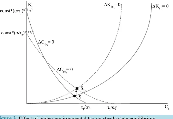
To see the long-term effect of an increase in environmental taxes, I look at the simultaneous effect of the shifts of both loci inFigure 3.
WhileFigure 3 suggests that the change in the equilibrium could be in either direction, the solution emerging from solving equations (10) and (11) provides an interesting analytical result4.
(
)
(
)
(
)
(
)
0 if
ˆ ˆ 0 if
1
0 if as 1
y y
y
y y
y
s C
s C
C C s C
C s C s
C s
τ γ
α γ τ
τ αγ τ γ
αγ α τ αγ τ αγ
< >
−
= > < <
− + − −
> < →
The tightening of environmental standards has two opposite effects. On one hand, it makes production asso-ciated with each unit of capital cleaner, so a higher capital stock becomes acceptable from the consumers’ pers-pective. On the other hand, a higher environmental tax lowers the marginal product of capital, lowering produc-tion. In equilibrium, the resource constraint identifies an equilibrium where the positive and negative forces balance each other. The derivative dC dτ is positive for lower values of
τ
. Starting at relatively low pollu-tion regulapollu-tion levels, the positive effect on capital outweighs the negative effect, i.e., an increasing environ-mental tax raises steady-state capital, production, and consumption. This happens because a higher emission tax makes higher capital stock acceptable, and the positive effect on production and consumption is stronger than the negative effect of the lower marginal product of each unit of this higher capital stock. The response of con-sumption and production to increases in environmental taxation turns negative whenτ
=syγ
C. Raising taxes beyond this level results in higher capital stocks’ positive effect on production and consumption being dominat-ed by the negative marginal product impact.The optimal emission tax is defined as the shadow cost of emissions to producers that equals the marginal disutility to consumers
τ
t=Pz t, =γ
Ct5. The incentive to raise steady-state consumption and production byraising the emission tax is not sufficient to drive the environmental tax to the optimal level; the relationship be-
872
Figure 2.Effect of higher environmental tax on steady state consumption locus.
Figure 3.Effect of higher environmental tax on steady state equilibrium.
tween production and the environmental tax turns negative before environmental taxes reach the optimal level except in the case of constant returns to scale
(
sy=1)
.3. Conclusions and Future Directions
[image:6.595.173.456.296.492.2]873
There are some aspects that need to be addressed in future work. For example, the environmental quality ad-dressed in this paper is a flow variable while many environmental quality variables are stock variables. Second, the international aspect both in terms of international spillovers of environmental externalities and international outsourcing of production are real-world complexities that need to be addressed in future extensions of this model.
References
[1] Bovenberg, A.L. and Smulders, S. (1995) Environmental Quality and Pollution Augmenting Technological Change in a Two Sector Endogenous Growth Model. Journal of Public Economics, 57, 369-391.
http://dx.doi.org/10.1016/0047-2727(95)80002-Q
[2] Bovenberg, A.L. and Smulders, S. (1996) Transitional Impacts of Environmental Policy in an Endogenous Growth Model. International Economic Review, 37, 861-893. http://dx.doi.org/10.2307/2527315
[3] Ono, T. (2003) Environmental Tax Policy and Long Run Economic Growth. Japanese Economic Review, 54, 203-217.
http://dx.doi.org/10.1111/1468-5876.00254
[4] Grimaud, A. and Rouge, L. (2014) Carbon Sequestration, Economic Policies and Growth. Resource and Energy
Eco-nomics, 36, 307-331. http://dx.doi.org/10.1016/j.reseneeco.2013.12.004
[5] Gupta, M.R. and Ray Barman, T. (2009) Fiscal Policies, Environmental Pollution and Economic Growth. Economic
Modelling, 26, 1018-1028. http://dx.doi.org/10.1016/j.econmod.2009.03.010
[6] Acemoglu, D., Aghion, P., Bursztyn, L. and Hemous, D. (2012) The Environment and Directed Technological Change.
American Economic Review, 102, 131-166. http://dx.doi.org/10.1257/aer.102.1.131
[7] Ramsey, F. (1928) A Mathematical Theory of Saving. Economic Journal, 38, 543-559.
http://dx.doi.org/10.2307/2224098
[8] Cass, D. (1965) Optimum Growth in an Aggregative Model of Capital Accumulation. Review of Economic Studies, 32, 233-240. http://dx.doi.org/10.2307/2295827
[9] Koopmans, T.C. (1965) On the Concept of Optimal Economic Growth. Econometric Approach to Development Plan-ning, North-Holland Publishing Company, Amsterdam, 225-287.
874
Appendix: Effect of Higher Environmental Tax on Steady State Consumption
Solve for steady-state consumption using Equations (10) and (11):1 1 1 1 1 1 1 1 1 y y s y s s C C α α α α α α α
α α γ α
α τ τ τ
α ρ − − − − − − − − − = −
{
}
1 1 1 1 11 1 1 1 1
ln ln ln ln 1
1 y 1 y y
C C
s s s
α
α α
α
α τ αγ α α α τ
τ α α ρ
− − − − − + − = − + − − − −
{
}
( )
1( )
( )
1 1
1 1 1 1
ln ln ln ln const
1 sy C 1 sy sy C sy
α
α α
α
τ αγ
α
τ
α
α
τ
α
α
− −
− − − − = − + − +
− − − −
{
}
( )
( )
( )
1 1 1
ln ln ln ln const
1 y 1 y y y
C C
s s s s
α
τ αγ
τ
α
α
τ
α
α
− − − = − + +
− − − −
Total differentiation of the above equation to see the effect of a change in environmental taxes on steady state consumption:
1 ˆ 1 1 ˆ
ˆ ˆ ˆ
1 y 1 y y y
C
C C
s PC C s s s
α τ τ αγ τ α α τ
τ αγ τ αγ α α
− − − = − +
− − − − − −
1 1 1 1 ˆ
ˆ
1 y 1 y y 1 y y
C
C
s C s s s C s
α τ α τ α αγ α
τ αγ α τ αγ α
− − − − − = + − − − − − − −
1 1 1 1
ˆ ˆ
1 y 1 y y 1 y y
C C
s C s s s C s
α τ α α αγ α
τ
τ αγ α τ αγ α
− − − = − − − − − − − − + −
(
)
(
)
(
)
(
)
ˆ ˆ 1 y y y s C CC s C s
α γ τ
τ
αγ α τ αγ