The exp( φ(ξ)) Expansion Method and Its Application for Solving Nonlinear Evolution Equations

http://dx.doi.org/10.4236/ijmnta.2015.41004

How to cite this paper: Abdelrahman, M.A.E., Zahran, E.H.M. and Khater, M.M.A. (2015) The exp

(

−ϕ ξ

( )

)

-Expansion Me-thod and Its Application for Solving Nonlinear Evolution Equations. International Journal of Modern Nonlinear Theory and

The exp

(

−

ϕ ξ

( )

)

-Expansion Method and Its

Application for Solving Nonlinear Evolution

Equations

Mahmoud A. E. Abdelrahman

1

, Emad H. M. Zahran

2

, Mostafa M. A. Khater

1*

1_{Department of Mathematics, Faculty of Science, Mansoura University, Mansoura, Egypt}

2_{Department of Mathematical and Physical Engineering, College of Engineering Shubra, Benha University,}

Egypt

Email: *[email protected]

Received 15 February 2015; accepted 6 March 2015; published 11 March 2015

Copyright © 2015 by authors and Scientific Research Publishing Inc.

This work is licensed under the Creative Commons Attribution International License (CC BY).

http://creativecommons.org/licenses/by/4.0/

Abstract

The exp

(

−φ ξ( )

)

-expansion method is used as the first time to investigate the wave solution of a

nonlinear dynamical system in a new double-Chain model of DNA and a diffusive predator-prey system. The proposed method also can be used for many other nonlinear evolution equations.

Keywords

The exp

(

−φ ξ( )

)

-Expansion Method, Dynamical System in a New Double-Chain Model of DNA, A

Diffusive Predator-Prey System, Traveling Wave Solutions, Solitary Wave Solutions, Kink-Anti Kink Shaped

1. Introduction

The nonlinear partial differential equations of mathematical physics are major subjects in physical science [1]. Exact solutions for these equations play an important role in many phenomena in physics such as uid mechanics, hydrodynamics, optics, plasma physics and so on. Recently many new approaches for finding these solutions have been proposed, for example, extended Jacobian Elliptic Function Expansion Method [2], the modified simple equation method [3], the tanh method [4], extended tended tanh-method [5]-[7], sine-cosine method

trigonometric function series method [18], G G ′    

 -expansion method [19]-[22], Jacobi elliptic function method

[23]-[26], the exp

(

−ϕ ξ

( )

)

-expansion method [27]-[29] and so on.

The objective of this article is to apply the exp

(

−ϕ ξ

( )

)

-expansion method for finding the exact traveling

wave solution of dynamical system in a new double-Chain model of DNA and a diffusive predator-prey system which play an important role in biology and mathematical physics.

The rest of this paper is organized as follows: In Section 2, we give the description of the exp

(

−ϕ ξ

( )

)

-ex-

pansion method. In Section 3, we use this method to find the exact solutions of the nonlinear evolution equations pointed out above. In Section 4, conclusions are given.

2. Description of Method

Consider the following nonlinear evolution equation

(

, _t, _x, _tt, _xx,

)

0,

F u u u u u  = (2.1)

where F is a polynomial in u x t

( )

, and its partial derivatives in which the highest order derivatives and nonlinear terms are involved. In the following,we give the main steps of this method:

Step 1. We use the wave transformation

( )

,

( )

, ,

u x t =u ξ ξ = −x ct (2.2)

where c is a positive constant, to reduce Equation (2.1) to the following ODE:

(

, , , ,

)

0,

P u u u u′ ′′ ′′′ = (2.3)

where P is a polynomial in u

( )

ξ and its total derivatives,while ' d '. dξ

=

Step 2. Suppose that the solution of ODE (2.3) can be expressed by a polynomial in exp

(

−ϕ ξ

( )

)

as follows

( )

_m

(

exp

(

( )

)

)

m , _m 0,

u ξ =a −ϕ ξ + a ≠ (2.4)

where ϕ ξ

( )

satisfies the ODE in the form

( )

exp

(

( )

)

exp

(

( )

)

,

ϕ ξ′ = −ϕ ξ +µ ϕ ξ +λ (2.5)

the solutions of ODE (2.5) are when λ2−₄µ>_0,

0,

µ

≠

( )

(

)

2 2

1

4 4 tanh

2

ln ,

2

C

λ µ

λ µ ξ λ

ϕ ξ

µ

  ₋  

− −  + − 

 

 _{ } 

=  

 

 

 

 

(2.6)

when 2

4 0, 0,

λ − µ> µ=

( )

₍

₍

₎

₎

1

ln ,

exp C 1

λ ϕ ξ

λ ξ

 

= − _ _

+ −

 

(2.7)

when λ2−₄µ=_{0, 0, 0,}µ≠ λ≠

( )

(

(

₍

1

)

₎

)

2

1

2 2

ln C ,

C λ ξ ϕ ξ

λ ξ

 + + 

= _− _

+

 

(2.8)

( )

ln

(

C1

)

,

ϕ ξ = ξ+ (2.9)

when λ2−4µ<0,

( )

(

)

2 2

1

4

4 tan

2

ln ,

2

C

µ λ

µ λ ξ λ

ϕ ξ

µ

  ₋  

 −  + − 

 

 _{ } 

=  

 

 

 

 

(2.10)

where am, , ,  λ µ are constants to be determined later,

Step 3. Substitute Equation (2.4) along Equation (2.5) into Equation (2.3) and collecting all the terms of the

same power exp

(

−mϕ ξ

( )

)

, m=0,1, 2, 3, and equating them to zero, we obtain a system of algebraic equa- tions, which can be solved by Maple or Mathematica to get the values of a_i.

Step 4. substituting these values and the solutions of Equation (2.5) into Equation (2.3) we obtain the exact solutions of Equation (2.3).

3. Application

3.1. Example 1: Dynamical System in a New Double-Chain Model of DNA

An attractive nonlinear model for the nonlinear science in the deoxyribonucleic acid (DNA). The dynamics of DNA molecules is one of the most fascinating problems of modern biophysics because it is at the basis of life. The DNA structure has been studied during last decades. The investigation of DNA dynamics has successfully predicted the appearance of important nonlinear structures. It has been shown that the nonlinearity is responsible for forming localized waves. These localized waves are interesting because they have the capability to transport energy without dissipation [30]-[38]. In Ref. [37] [38], it is given that a new double-chain model of DNA consists of two long elastic homogeneous strands which represent two polynucleotide chains of the DNA mole- cule, connected with each other by an elastic membrane representing the hydrogen bonds between the base pair of the two chains. Under some appropriate approximation, the new double-chain model of DNA can be des- cribed by the following two general nonlinear dynamical system:

2 3 2

1 1 1 1 1 ,

tt xx

u −c u =λu+γuv+µu +βuv (3.1)

2 2 2 3

2 2 2 2 2 0,

tt xx

v −c v =λ v+γ u +µ u v+β v +c (3.2)

where

(

)

(

)

1 2 1 0

0 0

2 1 2 2 1 2 3

0 0

1 2 3 0

2

; ; ;

2 2 2

2

; 2 ; ;

2 4

; .

Y F

c c c l

h

l l

h h

h l l

c h

µ λ

ρ ρ ρσ

µ µ

µ

λ γ γ µ µ

ρσ ρσ ρσ

µ µ

β β

ρσ ρσ

−

= ± = ± = −

− −

= = = = =

−

= = =

(3.3)

where

ρ

, σ , Y and F denote respectively the mass density, the area of transverse cross-section, the Young’s modulus and tension density of each strand;

µ

is the rigidity of the elastic membrance; h is the distance between the two strands, and l₀ is the height of the membrance in the equilibrium positive. In Equations (3.1) and (3.2), u is the difference of the longitudianl displacements of the bottom and top strands, while v is the difference of the transverse displacements of the bottom and top strands.

we first introduce the transformation

,

v=au b+ (3.4)

where a and b are constants, to reduce Equations (3.1) and (3.2) to the following system of equations:

(

)

(

)

(

)

2 3 2 2 2

1 1 1 2 1 1 1 1 1 ,

tt xx

and

(

)

(

)

3

2 3 2 2 2 2 2 2 2 0

2 2 2 3 2 2 3 2 .

tt xx

c

b b b

u c u u a u ab u b

a a a a a

γ µ λ β

µ β  β  λ β

− = + + _ + + _+ + + + +

  (3.6)

Comparing Equations (3.5) and (3.6) and using (3.4) we deduce that

2

h

b= and F=Y . Now Equations

(3.5) and (3.6) can be written as

2 3 2

1 0,

tt xx

u −c u −Au −Bu −Cu= (3.7)

where

(

2

)

0 2

1

3 2

0

6 2 2 6

2 4 ; a ; ; l ; Y.

A a B C c

l h

h h

µ

α

α

α

α

_α

ρσ

ρ

− 

= − + = =_ + _ = =

  (3.8)

The wave transformation u x t

( )

, =u

( )

ξ , ξ =kx+ωt, reduce Equation (3.7) to the following ODE:

(

2 2 2

)

3 2

1 0,

k c u Au Bu Cu

ω − ′′− − − = (3.9)

where 2 2 2

1 0

k c

ω − ≠ . Balancing u′′ and 3

u yields, N+ =2 3N→N=1. Consequently, we have the formal solution:

( )

0 1exp ,

u=a +a −ϕ (3.10)

where a₀ and a₁ are constants to be determined, such that a₁≠0. It is easy to see that

(

)

(

)

(

2

)

( )

1 1 1 1

2 exp 3 3 exp 2 2 exp ,

u′′ = a − ϕ + λa − ϕ +a λ + µ − +ϕ aλµ (3.11)

substituting Equation (3.10) and its derivatives in Equation (3.9) and equating the coefficient of different

power’s of exp

(

−ϕ ξ

( )

)

to zero, we get

(

2 2 2

)

3

1 1 1

2a w −c k −Aa =0, (3.12)

(

2 2 2

)

2 2 1 1 0 1 1

3λa w −c k −3Aa a −Ba =0, (3.13)

(

2

)(

2 2 2

)

2

1 2 1 3 0 1 2 0 1 1 0,

a λ + µ w −c k − Aa a − Ba a −Ca = (3.14)

(

2 2 2

)

3 2

1 1 0 0 0 0.

aλµ w −c k −Aa −Ba −Ca = (3.15)

Equations (3.12)-(3.15) yields

(

2 2 2

)

(

)

1 0 1 0

0 0 1 2

1

2

, , , ,

w c k a a a

a a a

A a

λ λ λ µ

− + ₋

= = − = =

2 2 2 2 2 2 2 2 2 2 2 2 2 2 2

0 1 0 1 1 0 0 1 1 1 1

2 1

4 4 4 4

,

a a w a a c k a w a c k w a c k a

C

a

λ − λ − + −λ +λ

= −

(

2 2 2 2 2 2

)

1 1 1 0 0 1 2

1

3 2 2

, .

a w a c k a w a c k

B A A

a

λ

λ

− + + −

= − =

Thus the solution is

(

2 2 2

)

_{( )}

1 0

2

exp

w c k

u a

A ϕ

− +

= ± − − (3.16)

( )

(

)

(

)

2 2 2

1 0 2 2 1 2 ₂ 4 4 tanh 2

w c k

u a A c µ ξ λ µ

λ µ ξ λ

− + = ±   ₋   − −  + −     _{ }    (3.17)

Case 2. if λ2−4µ>0, 0.µ=

( )

(

2 12 2

)

₍

₍

₎

₎

0

1

2

.

exp 1

w c k

u a A c λ ξ λ ξ − + = ±

+ − (3.18)

Case 3. if λ2−4µ=0, 0, 0.µ≠ λ≠

( )

(

2 12 2

)

₍

2

(

₎

1

)

0

1

2

.

2 2

w c k c

u a A c λ ξ ξ λ ξ − + ₊ = + +    

 (3.19)

Case 4. if λ2−4µ=0, 0, 0.µ= λ=

( )

(

2 12 2

)

_[

_]

0

1

2 ₁

.

w c k

u a A c ξ ξ − + = ±

+ (3.20)

Case 5. if λ2−4µ<0,

( )

(

)

(

)

2 2 2

1 0 2 2 1 2 ₂ . 4 4 tan 2

w c k

u a A c µ ξ µ λ

µ λ ξ λ

− + = ±   ₋    −  + −     _{ }    (3.21)

3.2. Example 2. A Diffusive Predator-Prey System

Consider a system of two coupled nonlinear partial differential equations describing the spatio-temporal dyna- mics of a predator-prey system [39],

(

)

2 3 3

1 ,

.

t xx

t xx

u u u u u uv

v v uv mv v

β β

κ δ

= − + + − −

= + − − (3.22)

where κ,

δ

, m and

β

are positive parameters. The solutions of predator-prey system have been studied in various aspects [39]-[41]. The dynamics of the diffusive predator-prey system have assumed the following

relations between the parameters, namely m=

β

and κ 1 β 1

δ

+ = + . Under there assumptions, Equation

(3.22) can be rewritten in the form:

2 3 3 1 , . t xx t xx

u u u u u uv

v v uv v v

β

κ

δ

κ

β

δ

 

= − +_ + _ − −

 

= + − −

(3.23)

We use the wave transformation u x t

( )

, =u

( )

ξ ξ, = −x ct to reduce Equation (3.23) to the following nonli- near system of ordinary differential equations:

2 3 3

1

0, 0,

u cu u u u uv

v cv uv v v

β

κ

δ

κ

β

δ

 _{′′+ ′− +} ₊  _{− − =}        ′′+ ′+ − − =  (3.24)

In order to solve Equation (3.24), let us consider the following transformation

1

v u

δ

= (3.25)

Substituting the transformation (3.25) into Equation (3.24), we get

2 3 ₀

u′′+cu′−βu+κu −u = (3.26)

Balancing u′′ with u3 in Equation (3.26) yields, N+ =2 3N⇒N=1. Consequently, we get the same formal solution (3.10). Substituting Equation (3.10) and its derivatives in Equation (3.26) and equating the coefficient of different power's of exp

(

−ϕ ξ

( )

)

to zero, we get

3

1 1

2a −a =0 (3.27)

2 2

1 1 1 0 1

3aλ−ca +κa −3a a =0 (3.28)

2 2

1 1 1 1 0 1 0 1

2aµ+aλ −caλ β− a +2κa a −3a a =0 (3.29)

3 3

1 1 0 0 0 0

aλµ−caµ β− a +κa −a = (3.30)

Equations (3.27)-(3.30) yields Case 1.

2 2

2

, 2 ,

2 2 4

c= κ β = µ−λ +κ λ λ=

0 1

2 1

, 2 2 2

a = ± λ+ κ a = ±

Case 2.

(

)

2

2 2

0 0 0 0 2

0 0 0

2 4 2

3 6 2 , 4

2

c a a a a

a a a

µ κµ

µ κ β µ κ

=_ − + + = − − + + +

(

2

)

0 0 0 1

0

2

2 , , 2

2a a a a a

λ= ± + µ = = ±

Thus the solution is Case 1.

( )

2 1

2exp 2 2

u= ± λ+ κ± −ϕ (3.31)

Case 2.

( )

0 2exp

u=a ± −

ϕ

(3.32)

Let us now discuss the following cases: Case 1.

Case (1.1). if 2

4 0, 0

λ − µ> µ≠

(

)

2 2

1

2 1 2 2

2 2 ₄

4 tanh 2

u

C

µ

λ κ

λ µ

λ µ ξ λ

= ± + ±

 ₋ 

 

− − + −

 

 

(3.33)

Case (1.2). if 2

4 0, 0

λ − µ> µ=

(

)

(

1

)

2 1 2

2 2 exp 1

u

C

λ

λ

κ

λ ξ

= ± + ±

+ − (3.34)

Case (1.3). if 2

4 0, 0, 0

(

)

(

)

(

)

2 1 1 2 2 1

2 2 2 2

C u C λ ξ λ κ λ ξ + = ± + + +

 (3.35)

Case (1.4). if λ2₋₄µ_{=0, 0, 0}µ₌ λ₌

1

2 1 2

2 2 u C λ κ ξ = ± + ±

+ (3.36)

Case (1.5). if λ2−₄µ<₀

(

)

2 2

1

2 1 2 2

2 2 ₄

4 tan 2 u C µ λ κ µ λ

µ λ ξ λ

= ± + ±  ₋    − + −     (3.37) Case 2.

Case (2.1). if λ2−4µ>0, 0µ≠

(

)

0 2 2 1 2 2 4 4 tanh 2 u a C µ λ µ

λ µ ξ λ

= ±  ₋    − − + −     (3.38)

Case (2.2). if 2

4 0, 0

λ − µ> µ=

(

)

(

)

0 1 2 exp 1 u a C λ λ ξ = ±

+ − (3.39)

Case (2.3). if λ2−4µ=0, 0, 0µ≠ λ≠

(

)

(

)

(

)

2 1 0 1 2 2 2 C u a C λ ξ λ ξ + = + +

 (3.40)

Case (2.4). if λ2₋₄µ_{=0, 0, 0}µ₌ λ₌

0 1 2 u a C ξ = ±

+ (3.41)

Case (2.5). if 2

4 0

λ − µ<

(

)

0 2 2 1 2 2 4 4 tan 2 u a C µ µ λ

µ λ ξ λ

= ±  ₋    − _ + _−   (3.42)

4. Conclusion

We establish exact solutions for the dynamics of DNA molecules is one of the most fascinating problems of modern biophysics because it is at the basis of life. The DNA structure has been studied during last decades. The investigation of DNA dynamics has successfully predicted the appearance of important nonlinear structures and a system of two coupled nonlinear partial differential equations describing the spatio-temporal dynamics of a

(a) (b)

(c) (d)

[image:8.595.72.499.75.693.2]

(e)

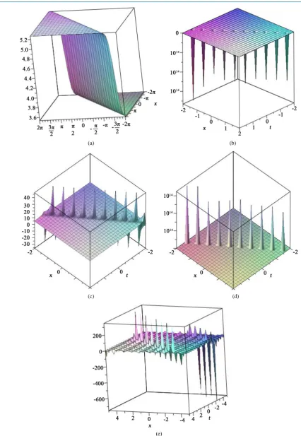
Figure 1. Solution of Equations (3.17)-(3.21). (a) Equations (3.17); (b) Equations (3.18); (c) Equations (3.19);

(a) (b)

(c) (d)

[image:9.595.110.492.77.696.2]

(e)

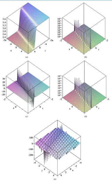
Figure 2. Solution of Equations (3.38)-(3.42). (a) Equations (3.38); (b) Equations (3.39); (c) Equations (3.40);

Double-Chain Model of DNA and a diffusive predator-prey system. It can be concluded that this method is reliable and proposes a variety of exact solutions NPDEs. The performance of this method is effective and can be applied to many other nonlinear evolution equations.

References

[1] Ablowitz, M.J. and Segur, H. (1981) Solitions and Inverse Scattering Transform. SIAM, Philadelphia.

[2] Zahran, E.H.M. and Khater, M.M.A. (2014) Exact Traveling Wave Solutions for the System of Shallow Water Wave Equations and Modified Liouville Equation Using Extended Jacobian Elliptic Function Expansion Method. American Journal of Computational Mathematics (AJCM), 4.

[3] Zahran, E.H.M. and Khater, M.M.A. (2014) The Modified Simple Equation Method and Its Applications for Solving Some Nonlinear Evolutions Equations in Mathematical Physics. Jokull Journal, 64.

[4] Wazwaz, A.M. (2004) The Tanh Method for Travelling Wave Solutions of Nonlinear Equations. Applied Mathematics and Computation, 154, 714-723. http://dx.doi.org/10.1016/S0096-3003(03)00745-8

[5] EL-Wakil, S.A. and Abdou, M.A. (2007) New Exact Travelling Wave Solutions Using Modified Extented Tanh-Func- tion Method. Chaos Solitons Fractals, 31, 840-852.

[6] Fan, E. (2000) Extended Tanh-Function Method and Its Applications to Nonlinear Equations. Physics Letters A, 277, 212-218.

[7] Abdelrahman, M.A.E., Zahran E.H.M. and Khater, M.M.A. (2015) Exact Traveling Wave Solutions for Modified Liouville Equation Arising in Mathematical Physics and Biology. International Journal of Computer Applications

(0975 8887), 112.

[8] Wazwaz, A.M. (2005) Exact Solutions to the Double Sinh-Gordon Equation by the Tanh Method and a Variable Sepa-rated ODE Method. Computers & Mathematics with Applications, 50, 1685-1696.

http://dx.doi.org/10.1016/j.camwa.2005.05.010

[9] Wazwaz, A.M. (2004) A Sine-Cosine Method for Handling Nonlinear Wave Equations. Mathematical and Computer Modelling, 40, 499-508. http://dx.doi.org/10.1016/j.mcm.2003.12.010

[10] Yan, C. (1996) A Simple Transformation for Nonlinear Waves. Physics Letters A, 224, 77-84.

http://dx.doi.org/10.1016/S0375-9601(96)00770-0

[11] Fan, E. and Zhang, H. (1998) A Note on the Homogeneous Balance Method. Physics Letters A, 246, 403-406.

http://dx.doi.org/10.1016/S0375-9601(98)00547-7

[12] Wang, M.L. (1996) Exact Solutions for a Compound KdV-Burgers Equation. Physics Letters A, 213, 279-287.

http://dx.doi.org/10.1016/0375-9601(96)00103-X

[13] Abdou, M.A. (2007) The Extended F-Expansion Method and Its Application for a Class of Nonlinear Evolution Equa-tions. Chaos, Solitons & Fractals, 31, 95-104. http://dx.doi.org/10.1016/j.chaos.2005.09.030

[14] Ren, Y.J. and Zhang, H.Q. (2006) A Generalized F-Expansion Method to Find Abundant Families of Jacobi Elliptic Function Solutions of the (2+1)-Dimensional Nizhnik-Novikov-Veselov Equation. Chaos, Solitons & Fractals, 27, 959-979. http://dx.doi.org/10.1016/j.chaos.2005.04.063

[15] Zhang, J.L., Wang, M.L., Wang, Y.M. and Fang, Z.D. (2006) The Improved F-Expansion Method and Its Applications.

Physics Letters A, 350, 103-109. http://dx.doi.org/10.1016/j.physleta.2005.10.099

[16] He, J.H. and Wu, X.H. (2006) Exp-Function Method for Nonlinear Wave Equations. Chaos, Solitons & Fractals, 30, 700-708. http://dx.doi.org/10.1016/j.chaos.2006.03.020

[17] Aminikhad, H., Moosaei, H. and Hajipour, M. (2009) Exact Solutions for Nonlinear Partial Differential Equations via Exp-Function Method. Numerical Methods for Partial Differential Equations, 26, 1427-1433.

[18] Zhang, Z.Y. (2008) New Exact Traveling Wave Solutions for the Nonlinear Klein-Gordon Equation. Turkish Journal of Physics, 32, 235-240.

[19] Wang, M.L., Zhang, J.L. and Li, X.Z. (2008) The G

G ′    

 -Expansion Method and Travelling Wave Solutions of

Nonli-near Evolutions Equations in Mathematical Physics. Physics Letters A, 372, 417-423.

http://dx.doi.org/10.1016/j.physleta.2007.07.051

[20] Zhang, S., Tong, J.L. and Wang, W. (2008) A Generalized G

G ′    

 -Expansion Method for the mKdv Equation with

[21] Abdelrahman, M.A.E., Zahran, E.H.M. and Khater, M.M.A. (2015) Exact Traveling Wave Solutions for Modified Liouville Equation Arising in Mathematical Physics and Biology. International Journal of Computer Applications

(0975 8887), 112.

[22] Zahran, E.H.M. and Khater, M.M.A. (2014) Exact Solutions to Some Nonlinear Evolution Equations by Using (G’/G)-Expansion Method. Jokull Journal, 64.

[23] Dai, C.Q. and Zhang, J.F. (2006) Jacobian Elliptic Function Method for Nonlinear Differential Difference Equations.

Chaos, Solitons & Fractals, 27, 1042-1049. http://dx.doi.org/10.1016/j.chaos.2005.04.071

[24] Fan, E. and Zhang, J. (2002) Applications of the Jacobi Elliptic Function Method to Special-Type Nonlinear Equations.

Physics Letters A, 305, 383-392. http://dx.doi.org/10.1016/S0375-9601(02)01516-5

[25] Liu, S., Fu, Z., Liu, S. and Zhao, Q. (2001) Jacobi Elliptic Function Expansion Method and Periodic Wave Solutions of Nonlinear Wave Equations. Physics Letters A, 289, 69-74. http://dx.doi.org/10.1016/S0375-9601(01)00580-1

[26] Zhao, X.Q., Zhi, H.Y., Zhang, H.Q. (2006) Improved Jacobi-Function Method with Symbolic Computation to Con-struct New Double-Periodic Solutions for the Generalized Ito System. Chaos Solitons Fractals, 28, 112-126.

[27] Abdelrahman, M.A.E., Zahran, E.H. M. and Khater, M.M.A. (2014) Exact Traveling Wave Solutions for Power Law and Kerr Law Non Linearity Using the Exp

(

ϕ η

( )

)

-Expansion Method. GJSFR, Volume 14, Issue 4, Version 1.0. [28] Mahmoud A.E. Abdelrahman and Mostafa M.A. Khater (2015) The Exp

(

ϕ η

( )

)

Expansion Method and Its

Appli-cation for Solving Nonlinear Evolution Equations. International Journal of Science and Research (IJSR), 4, 2319-7064.

[29] Khan, K. and Akbar, M.A. (2014) Solitary Wave Solutions of Some Coupled Nonlinear Evolution Equations. Journal of Scientific Research, 6, 273-284

[30] Aguero, M., Najera, M. and Carrillo, M. (2008) Non Classic Solitonic Structures in DNA’s Vibrational Dynamics. In-ternational Journal of Modern Physics B, 22, 2571-2582. http://dx.doi.org/10.1142/S021797920803968X

[31] Gaeta, G. (1999) Results and Limitations of the Soliton Theory of DNA Transcription. Journal of Biological Physics,

24, 81-96. http://dx.doi.org/10.1023/A:1005158503806

[32] Gaeta, G., Reiss, C., Peyrard, M. and Dauxois, T. (1994) Simple Models of Nonlinear DNA Dynamics. La Rivista Del Nuovo Cimento Series 3, 17, 1-48. http://dx.doi.org/10.1007/BF02724511

[33] Yakushevich, L.V. (1987) Nonlinear Physics of DNA. Studio Biophys, 121, 201.

[34] Yakushevich, L.V. (1989) Nonlinear DNA Dynamics: A New Model. Physics Letters A, 136, 413-417.

http://dx.doi.org/10.1016/0375-9601(89)90425-8

[35] Yakushevich, L.V. (1998) Nonlinear Physics of DNA. Wiley and Sons, England.

[36] Peyrard, M. and Bishop, A. (1989) Statistical Mechanics of a Nonlinear Model of DNA Denaturation. Physical Review Letters, 62, 2755-2758. http://dx.doi.org/10.1103/PhysRevLett.62.2755

[37] Kong, D.X., Lou, S.Y. and Zeng, J. (2001) Nonlinear Dynamics in a New Double Chain-Model of DNA. Communica-tions in Theoretical Physics, 36, 737-742. http://dx.doi.org/10.1088/0253-6102/36/6/737

[38] Alka, W., Goyal, A. and Kumar, C.N. (2011) Nonlinear Dynamics of DNA-Riccati Generalized Solitary Wave Solu-tions. Physics Letters A, 375, 480-483. http://dx.doi.org/10.1016/j.physleta.2010.11.017

[39] Petrovskii, S.V., Malchow, H. and Li, B.L. (2005) An Exact Solution of a Diffusive Predator-Prey System. Proceed-ings of the Royal Society A, 461, 1029-1053.

[40] Kraenkel, R.A., Manikandan, K. and Senthivelan, M. (2013) On Certain New Exact Solutions of a Diffusive Preda-tor-Prey System. Communications in Nonlinear Science and Numerical Simulation, 18, 1269-1274.

http://dx.doi.org/10.1016/j.cnsns.2012.09.019

[41] Dehghan, M. and Sabouri, M. (2013) A Legendre Spectral Element Method on a Large Spatial Domain to Solve the Predator-Prey System Modeling Interaction Populations. Applied Mathematical Modeling, 37, 1028-1038.