Crank-Nicolson Implicit Method For The Nonlinear
Schrodinger Equation With Variable Coefficient
Yaan Yee Choy
a, Wooi Nee Tan
b, Kim Gaik Tay
cand Chee Tiong Ong
daFaculty of Science, Technology & Human Development, Universiti Tun Hussein Onn Malaysia,
86400 Parit Raja, Batu Pahat, Johor.
bFaculty of Engineering, Multimedia University, 63100 Cyberjaya, Selangor. cFaculty of Electrical & Electronic Engineering, Universiti Tun Hussein Onn Malaysia,
86400 Parit Raja, Batu Pahat.
dFaculty of Science, Universiti Teknologi Malaysia, 81310 Skudai, Johor.
Abstract. In the present work, the Crank-Nicolson implicit scheme for the numerical solution of nonlinear Schrodinger equation with variable coefficient is introduced. The Crank-Nicolson scheme is second order accurate in time and space directions. The stability analysis for the Crank-Nicolson method is investigated and this method is shown to be unconditionally stable. The numerical results obtained by the Crank-Nicolson method are presented to confirm the analytical results for the progressive wave solution of nonlinear Schrodinger equation with variable coefficient.
Keywords: Crank-Nicolson implicit method, nonlinear Schrodinger equation with variable coefficient, stability, maximum absolute error.
PACS: 02.60.-x, 02.60.Lj, 02.70.Bf
INTRODUCTION
Consider the following nonlinear Schrodinger (NLS) equation with variable coefficient [1],
2
2
1 2 2 3 1 0,
,0 , , , , 0, 0 ,
, 0, 1,
U U
i U U h U
U a b
U a U b T
i
P P P W
W [
W W W
[ [ [
W [
)
w w
w w
, [!0,
(1)
where the coefficients of
P P
1, and 2P
3 are nonzero values. Equation (1) is in dimensionless form where,
U U W [ is a complex value function. The second term and the forth term represent the dispersion effect and the variable coefficient, respectively. The third term is the nonlinear term which measures the strength of the nonlinearity relative to wave dispersion. The nonlinearity is focusing when
P
2!!0 and defocusing whenP
20. The ) W is a smooth function which decreases exponentially for sufficiently large W .When
P
3 equals to zero, the equation (1) is well known as the nonlinear Schrodinger (NLS) equation. The NLSequation is the simplest representative equation describing the self-modulation of one-dimensional monochromatic plane waves in dispersive media [2]. The NLS equation appears in many branches of physics and applied mathematics. Recently, the mathematical modeling of blood flow through a stenosed artery governed by the NLS equation has been studied by several researchers [3]-[5]. This equation describes the modulation of amplitude waves in a thin stenosed elastic tube. The study of the effect of stenosis on blood flow in arteries becomes important since the NLS equation is able to describe and give a better understanding of the dynamics of the circulatory system in the human body and give more insight into the medical field.
Since the analytical solutions for the NLS equation are limited, numerical methods have become important in order to understand the physical behavior of the equation. Many researchers are devoted to study the numerical solution of NLS equation. Numerous numerical methods have been investigated such as the discrete Adomian decomposition [7], the finite difference [8], the finite element [9] and the multi-symplectic Runge-Kutta [10].
In the present work, we proposed the Crank-Nicolson implicit method for solving the NLS equation with variable coefficient. The truncation errors for the present method are second order in time and space directions. The stability analysis shows that the present method is unconditionally stable and satisfies discrete conservation laws. The numerical results obtained by the present method are compared with the exact solutions [1]. It shows that the Crank-Nicolson method is compatible with the analytical result.
Our paper is organized as follows: in Section 2, we will introduce the Crank-Nicolson implicit method to solve the NLS equation with variable coefficient. We investigated the stability analysis for equation (1) in Section 3. In Section 4, we present the numerical results and compared them with the analytical results. Section 5 ends this paper with a conclusion.
THE CRANK-NICOLSON IMPLICIT METHOD
The analytical solution of the equation (1) mention U as a function of [ and W , U W [, where both [ and W
are continuous variables. For the finite difference method, we seek approximation n m
U to the original function ,
U
W [
at a set of points[
m,W
n on a rectangular grid in the 2-dimensional plane, [ and W , where[
m[
0m'[
,
W
nW
0 n'W
, '[ and 'W are the grid spacing in [ and W , respectively. For simplicity,[
0 andW
0 are set to be0 0
[
andW
0 0 in our following discussion.The main idea of Crank-Nicolson implicit method is to produce the same order of truncation error in W and [
variables. For this reason, the forward difference for W derivative in equation (1) is replaced with the backward difference approximation, this gives
22
, , , ,
, 2
U W [ U W [ U W W [ W U y[
W W W
' '
'
w w
w w (2)
for some y in
W
'W W
, . The [ derivative in equation (1) is the usual central difference approximation, 22 4
2
2 4
, , 2 , , ,
, 12
U W [ U W [ [ U W [ U W [ [ [ U W x
[ [ [
' ' '
'
w w
w w (3)
for some x in
[
'[ [
, '[
. Then the equation (1) can be written as1
2
1 1
1 2 2 3 1
2
0, , 1,...,0,1,..., , 0,1, 2,..., .
n n n n n
n n n
m m m m m
m m m
U U U U U
i U U h U
for m M M M n N
P P P W
W [
' '
ª º
ª º
« »
« »
« »
¬ ¼ ¬ ¼
(4)
Equation (4) is the implicit backward difference equation at the nth step in W with the truncation error of order
2O W [ . For the backward difference equation at the
n1 th step in W , the equation (4) becomes1 1 1 1
2
1 1 1
1 1
1 2 2 3 1
2
0, , 1,...,0,1,..., , 0,1, 2,..., .
n n n n n
n n n
m m m m m
m m m
U U U U U
i U U h U
for m M M M n N
P P P W
W [
' '
ª º
ª º
« »
« »
« »
¬ ¼ ¬ ¼
(5)
1 1 1 1
2 12 1 1
1 1 1 1 3
1 2
1
2 2
2 2
0,
2 2 2
, 1,...,0,1,..., , 0,1, 2,..., ,
n n n n n n n n
n n n n n n
m m m m m m m m
m m m m m m
U U U U U U U U
i U U U U h U U
for m M M M n N
P
P P W
W [ [
' ' '
ª º
ª º ª º
« » ª º
« » « » ¬ ¼ ¬ ¼
¬ ¼ ¬ ¼
(6) where the truncation error is of order
2 2O W [ . Rearrange the above expression, yield the difference equation for the Crank-Nicolson implicit method:
1 3 1 1
1 1
1 1 1 1
2 12 1
3
1 2
1 1 1 1
2 2 2
,
2 2 2
n n n
m m m
n n n n n n n
m m m m m m m
rU i r h U rU
r U U i r h U U U U U
P
P P W W P
P
P P W W P W
'
' '
ª º
« »
¬ ¼
ª º ª º
ª º
¬ ¼ « » ¬ ¼
¬ ¼
(7)
with r 2
W [
' ' .
The solution for the above difference equation (7) is sought in the region
M'[ [d mdM'[ u WndN'W, ,...,m M M , n 0,1,2,...,N. Since equation (1) is a boundary value problem, so the values of U at time, [ step, n 0 are known. The right-hand side of equation (7) consists of both of the known values U at time step n
as well as the unknown values U at time step n1. In order to solve the above equation (7), we apply the Functions Arguments which can be referred to using MATLAB package.
STABILITY ANALYSIS
In this section, we investigate the stability analysis of the Crank-Nicolson implicit method that we have discussed in Section 2. First, we linearized the NLS equation with variable coefficient (1). We later obtained the difference equation by applying the Crank-Nicolson implicit method to the linearized NLS equation. To analyze the stability of the numerical scheme, we use Fourier series method which leads to the analysis known as von-Neumann stability test.
The most common linearization methods are Taylor's series expansion, optimal linearization method and global linearization method. In this paper, we adopt the method of Taylor's series expansion. Consider the function f U
of a single variable U . Suppose that U is a point such that f U 0. The point U is called equilibrium point of the system *
U f U . By expanding the NLS equation with variable coefficient (1) in Taylor series expansion of
f U , this gives the linearized NLS equation with variable coefficient,
* 2 *
*
1 2* 3 0.
U U
i P PU
W [
w w
w w (8)
Employing the Crank-Nicolson implicit method to the linearized NLS equation with variable coefficient (8), we have the difference equation,
* 1 3 * 1 * 1 * 3 * *
1 1 1 1
1 1 1 1 1 1,
2 2 2 2 2 2
n n n n n n
m m m m m m
rU i r P U rU rU i r P U rU
P P P P
P 'W P 'W
ª º ª º
« » « »
¬ ¼ ¬ ¼ (9)
with r 2
W [
'
' . For the von-Neumann method, a harmonic decomposition is made of the error E at grid points at a given time level, leading to the error function
,
i x j j
j
where the frequencies Ej and j are arbitrary. To investigate the error propagation as time increases, it is
necessary to find a solution of the finite difference equation which reduces to ei xE when time is zero. Apply
equation (10) into equation (9) and the n m
E satisfies the same finite difference equation, so we get
1 3 1 1 3
1 1 1 1
1 1 1 1 1 1.
2 2 2 2 2 2
n n n n n n
m m m m m m
rE i r P E rE rE i r P E rE
P P 'W P P P 'W P
ª º ª º
« » « »
¬ ¼ ¬ ¼ (11)
Substitute n nk i mh m
E e eD E , equation (11) becomes
1 1 3 1 1 1
1 1
1
1 3 1
1 1
1
2 2 2
.
2 2 2
n k i m h n k i mh n k i m h
i m h i m h
nk nk i mh nk
re e i r e e re e
re e i r e e re e
D E D E D E
E E
D D E D
P
P P W P
P
P P W P
'
'
ª º
« »
¬ ¼
ª º
« »
¬ ¼
(12)
Cancellation of e eDnk i mhE leads to
2 3
1
2 3
1
2 sin
2 2 .
2 sin
2 2
k
h
i r
e
h
i r
D
P W P E
P W P E
'
'
§ ·
¨ ¸
© ¹
§ ·
¨ ¸
© ¹
(13)
The quantity, eDk is called the amplification factor. For stability, eDk d1, for all values of
E
h. Clearly, themodulus is at most one for all positive values of r. Thus, the Crank-Nicolson implicit method is unconditionally stable according to linear analysis. However, in the actual condition, the simulation may become unstable because nonlinear terms may play a dominant role in the dynamics.
RESULTS & DISCUSSION
In this section, we apply the scheme of equation (7) to solve equation (1). Furthermore, we also compared our proposed Crank-Nicolson implicit method with the exact solution of NLS equation with variable coefficient. In comparing the numerical results with the exact results, we calculate the maximum absolute error, Lff at certain
[
mwhich is defined as
max exact numerical .
Lf U U (14)
The exact solution for the NLS equation with variable coefficient (1) is given by [1]
1/2
2
3 1
1 0
, tanh exp ,
2
U a a i K h s ds
W
P
W [ 9 [ W P
P :
ª§ · º ª § ·º
«¨ ¸ » « ¨¨ ¸¸»
«© ¹ » «¬ © ¹»¼
¬ ¼
³
(15)
where
] [
2P W
1K and2 2
1K 2a
P P
: . The coefficients of P P1, and 2 P3 can be obtained in [1]. The h1 W
is the stenosis function which is defined as sech 0.30
W
. In order to obtain a numerical solution, we need the initial condition by assuming (1)W
0 in equation (15), (2) spatial step,W
0.01,(3) travelling wave profile step,0.01
[ and (4) artificial boundary conditions, U
W
, 2 UW
,5 0. The numerical results are presented over the travelling wave profile interval>>
2,5@
and the space interval>>
6,1@
by choosing the parameter as a 1, K 2.TABLE (1). Maximum absolute errors of the NLS equation with variable coefficient (1) at '
W
0.01, ' [ 0.01 for different [.Travelling wave profile, [ 0.0 1.0 1.50 2.00 2.50 3.00
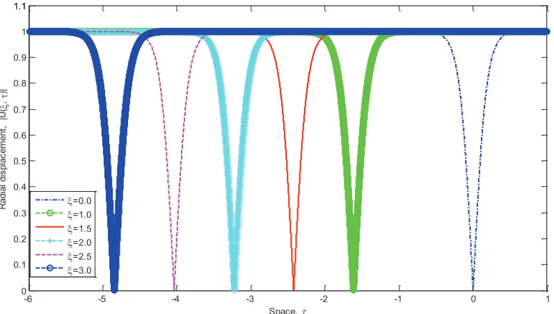
[image:4.612.74.541.653.683.2]FIGURE 1. Crank-Nicolson solution of the NLS equation with variable coefficient (1) with space W at certain travelling wave profile [.
FIGURE 2. Exact solution of the NLS equation with variable coefficient (1) with space W at certain travelling wave profile
[.
The maximum absolute errors, Lff between the exact and numerical solutions of the NLS equation with variable
coefficient are shown in Table (1). Figure 1 depicts the Crank-Nicolson implicit solution for the NLS equation with variable coefficient. It is seen that the numerical solution in Figure (1) is exactly the same as the exact solution in Figure (2) in terms of position and amplitude.
-6 -5 -4 -3 -2 -1 0 1 0
0.1 0.2 0.3 0.4 0.5 0.6 0.7 0.8 0.9 1 1.1 1.1
R
ad
ia
l d
is
pl
ac
em
en
t, |
U
(W , [
)|
Space, W
[=0 [=1.0 [=1.5 [=2.0 [=2.5 [=3.0
-6 -5 -4 -3 -2 -1 0 1 0
0.1 0.2 0.3 0.4 0.5 0.6 0.7 0.8 0.9 1 1.1 1.1
R
ad
ia
l d
is
pl
ac
em
en
t, |
U
([ , W
)|
Space, W [=0.0
TABLE (2). Maximum absolute errors of the NLS equation with variable coefficient (1) at '
W
0.01, ' [ 0.01 for different W .Space, W -6 -4 -2 0 1
Lff 0.4403 0.2839 0.2462 0.0000 0.0703
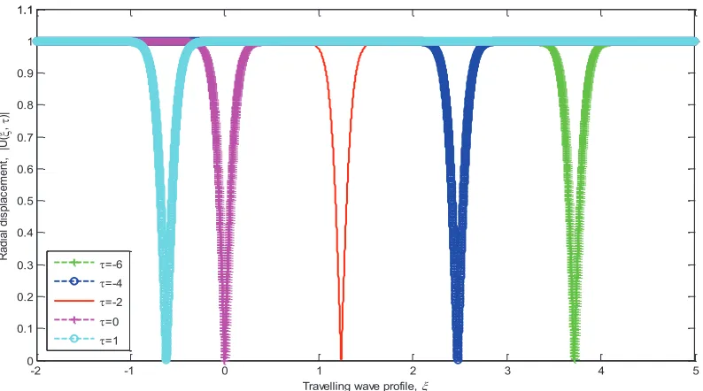
[image:6.612.117.526.90.390.2]FIGURE 3. Crank-Nicolson solution of the NLS equation with variable coefficient (1) with travelling wave profile [ at certain space W .
FIGURE 4. Exact solution of the NLS equation with variable coefficient (1) with travelling wave profile [ at certain space
W .
-2 -1 0 1 2 3 4 5 0
0.1 0.2 0.3 0.4 0.5 0.6 0.7 0.8 0.9 1 1.1 1.1
R
ad
ia
l d
is
pl
ac
em
en
t, |
U
( [ , W
)|
Space, [ W=-6
W=-4 W=-2 W=0 W=1
-2 -1 0 1 2 3 4 5 0
0.1 0.2 0.3 0.4 0.5 0.6 0.7 0.8 0.9 1 1.1 1.1
R
ad
ia
l d
is
pl
ac
em
en
t, |
U
([ , W
)|
Travelling wave profile, [ W=-6
[image:6.612.128.525.460.681.2]Table (2) illustrates the maximum absolute errors, Lff between the numerical and exact solutions of the NLS
equation with variable coefficient with different W . The maximum absolute errors in Tables (1) and (2) are quite large for most of the cases. This is due to the number of spatial grid points are less and the step size of travelling wave profile is large. In Table (2), for
W
0,
the maximum error is small because it is the initial condition. To maintain the stability and to achieve the high accuracy of the approximation solution, the number of spatial grid points must be large and the step size of travelling wave profile must be small. However, this numerical scheme required large computational cost if number of grid points for spatial or travelling wave profile increases. Comparing Figures 3 and 4, it is shown that the numerical results show good approximation with the analytical results. However, this numerical scheme required extremely large computational cost.CONCLUSION
The Crank-Nicolson implicit method with second order accurate in time and space direction is proposed for solving the NLS equation with variable coefficient. This method is shown to be unconditionally stable for the linearized NLS equation with variable coefficient. Numerical tests presented for the NLS equation with variable coefficient show that our method is in agreement with the analytical method.
ACKNOWLEDGEMENTS
The authors gratefully acknowledge financial support from the Registrar Office, UTHM.
REFERENCES
1. Y.Y. Choy, C.T. Ong and K.G. Tay, Mathematics Journal of Universiti Teknologi Malaysia28, 1-13 (2012). 2. H. Demiray, J. of Maths. and Math. Sci. 60, 3205-3218 (2004).
3. G.K. Tay, Y.Y. Choy, C.T. Ong and H. Demiray, Int. J. Eng. Sci. and Tech. 2, 708-723 (2010). 4. H. Demiray, Int. J. Eng. Sci. 36, 1061-1082 (1998).
5. H. Demiray, Int. J. Eng. Sci.41, 1387-1403 (2003).
6. H. Demiray, Applied Maths. And Computation145, 179-184 (2003).
7. A. Bratsos, M. Ehrhardt and I.T. Famelis, Applied Maths. And Computation197, 190-205 (2008). 8. M. Dehghan and A. Taleei, Computer Physics Communications181, 43-51 (2010).
9. J. Argyris and M. Haase, Comput. Methods Appl. Mech. Engrg61, 71-122 (1987). 10. S. Reich, J. Comput. Phys.157, 473-499 (2000).