Minimization of the Difference between the Theoretical
Mean of the Rayleigh Probability Density Function and
the Mean Obtained from its Plot
Mustafa Mutlu
Teknik Bilimler MYO Ordu University 52200, Ordu, Turkey *Corresponding Author: [email protected]
Copyright © 2014 Horizon Research Publishing All rights reserved
Abstract
In this study, the difference between the mean of the Rayleigh Probability Density Function and the mean obtained from the graph of Rayleigh Probability Density Function is minimized by changing the coefficient in the equation yielding the mean. By using various numbers of data and K values, Rayleigh Probability Density Function is plotted with the means mentioned above.Keywords
Rayleigh Probability Density Function, Line of Sight, No Line of Sight1. Introduction
Rayleigh Probability Density Function is used for the cases in which there is NLOS between transmitters and receivers for the communication networks and channel modeling. When there occur phase differences between multipath signals arriving the receiver, fading takes place. Rayleigh distribution function is used for multipath fading in modeling of change of voltage or power that will be received[1-8]. In Rayleigh modeling, in contrast to the Ricean, there is no any specified direction, that is, signals coming from any direction are assumed to have equal probability.
Moreover Rayleigh Modeling is used for noise analysis. If a signal coming to a receiver via reflection becomes so greater than the direct signal that it suppresses that, in this case this type of channel modeling is done by means of Rayleigh Probability Density Function.
The aim of our study is to find an expression which results in numerical values that are very close to the actual values. For this purpose after much iteration we have obtained a new coefficient that gives the desired results.
2. Theory
Rayleigh Probability Density Function changes with
respect to a single parameter, either standard deviation or K[9-15]where K is the power of direct signal divided by the power of coming signal via reflection and expressed as
𝐾𝐾=𝑃𝑃′𝑙𝑙𝑙𝑙𝑙𝑙 𝑃𝑃⁄ ′𝑚𝑚𝑚𝑚𝑙𝑙𝑚𝑚𝑚𝑚𝑚𝑚𝑚𝑚𝑚𝑚ℎ (1)
𝐾𝐾= 1 2 ⁄ 𝜎𝜎2 (2)
𝑃𝑃′
𝑙𝑙𝑙𝑙𝑙𝑙 = 0 𝑊𝑊𝑚𝑚𝑚𝑚𝑚𝑚= 1 𝑑𝑑𝑑𝑑𝑊𝑊 (3)
K characterizes the environment. K values are normalized when using in the equation(4).
Rayleigh Probability Density Function is expressed as 𝑓𝑓𝑧𝑧(𝑧𝑧) = 2 𝑧𝑧𝐾𝐾𝑒𝑒𝑒𝑒𝑚𝑚�(−𝑧𝑧2𝐾𝐾)� (4)
When K represents the Power
L = K 10⁄ (5)
and if it represents the voltage
𝐿𝐿=𝐾𝐾⁄20 (6)
is used. For both cases,
𝑆𝑆= 10𝐿𝐿. (7)
Normalized Rayleigh Probability Density Function can be written as
𝑓𝑓𝑧𝑧(𝑧𝑧) = 2 𝑧𝑧𝑆𝑆𝑒𝑒𝑒𝑒𝑚𝑚�(−𝑧𝑧2𝑆𝑆)� (8)
S is obtained through the equations (5), (6), (7) and used in equation (8) to obtain fz(z).
Mean of this function is
𝑓𝑓𝑧𝑧(𝑧𝑧)(𝑚𝑚𝑒𝑒𝑚𝑚𝑚𝑚) =𝑀𝑀[𝑧𝑧] =∫ 𝑧𝑧0∞ 𝑓𝑓𝑧𝑧(𝑧𝑧) 𝑑𝑑𝑧𝑧, (9)
And theoretical mean can be written as,
𝑇𝑇𝑀𝑀=𝑀𝑀[𝑧𝑧] =�12� �𝜋𝜋/𝐾𝐾= 1.2533𝜎𝜎 (10) And the variance is written as
And the Standard deviation is
𝜎𝜎= 0.4632/√𝐾𝐾 (12)
[image:2.595.62.297.156.313.2]Table 1 shows the actual and theoretical means and percent error of theoretical mean.
Table 1. Actual and Theoretical Mean Values and Percent Errors.
for 171 data K voltage (dB) AM Actual mean TM
theoretical mean Error(%)
10 41 49.83 5.16
12 36 44.44 4.93
14 33 39.58 3.84
16 29 35.28 3.67
18 26 31.44 3.18
20 23 28.02 2.93
3. Modification of Theoretical Mean
Expression
In equation (10) the coefficient ½ is not suitable. Because there is a big difference between the actual and theoretical curves when theoretical mean is used for the plot of Rayleigh Probability Density Function. Instead we suggest a change in equation (10) to achieve more reasonable results. After many iterations the coefficient ½ is replaced by 1/2.3589 to minimize the difference between the theoretical mean(TM) and the actual mean (AM) which is obtained from the graph of Rayleigh Probability Density Function.
Since TM being a function of K is the theoretical mean, if and only if K1 is used instead of K in Rayleigh Probability Density Function its actual mean becomes TM. This is illustrated in Table 4.
Equation (14) can be used for finding K1 by replacing it in place of K.
f1(z) = 2 𝑧𝑧𝐾𝐾1 𝑒𝑒𝑒𝑒𝑚𝑚�(−𝑧𝑧2𝐾𝐾1)� (13)
𝑀𝑀𝑀𝑀=𝑀𝑀1[𝑧𝑧] =�2.35891 � �𝜋𝜋/𝐾𝐾 (14)
[image:2.595.313.552.229.386.2]Where MM is the modified mean. As can be seen from Table1, and Table 2 for K=10 dB AM=41, TM=49.83 MM=42 is obtained. This shows that the equation (14) yields a value which is very close to the actual mean whereas the theoretical one (TM) is far from it.
Table 2. Actual and Modified Mean Values and Percent Errors
for 171 data K voltage (dB) AM Actual mean MM
Modified mean Error (%)
10 41 42 0.58
12 36 37 0.58
14 33 33.56 0.32
16 29 30 0.58
18 26 26.6 0.35
20 23 23.76 0.44
Since the variance and standard deviation values are derived from the mean, an erroneous mean causes wrong results in variance and standard deviation[16-23]. Therefore to obtain minimum difference between the actual and theoretical mean, we changed the coefficient value several times. As a result we reduced the percent error from 5.16 percent to 0.32 percent. The average of x number of data can be expressed as
𝑀𝑀𝑀𝑀𝑒𝑒=𝐷𝐷𝑚𝑚𝑚𝑚𝑚𝑚171 𝑒𝑒𝑀𝑀𝑀𝑀171 (15)
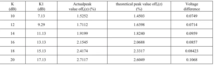
[image:2.595.93.520.567.697.2]Where MM171 is the average value of 171 data. In Table 3 peak values corresponding to AM and TM voltage differences (errors) are given.
Table 3. Actual and Theoretical Peak Values and the difference between them K
(dB) (dB) K1 value offActualpeak z(z) (%)
theoretical peak value offz(z)
(%) difference Voltage
10 7.13 1.5252 1.4503 0.0749
12 9.29 1.7112 1.6398 0.0714
14 11.13 1.9199 1.8240 0.0959
16 13.13 2.1545 2.0688 0.0857
18 15.13 2.4174 2.3317 0.08423
Table 4 shows the variations of fz(z) and f1z(z)..
Table 4. fz(z) and f1z(z) values depending on K and K1 respectively
K(dB) fz(z)=2 z Sexp(-z2S) K1(dB) f1z(z) =2 z S1exp(-z2S1)
10 6.32 z exp(-z23.16) 7.13 4.54 zexp(-z22.27)
12 7.96 z exp(-z23.98) 9.29 5.82 z exp(-z22.91)
14 10.02 z exp(-z25.01) 11.13 7.20 z exp(-z23.60)
16 12.61 z exp(-z26.30) 13.13 9.06zexp(-z24.53)
18 15.88 zexp(-z27.94) 15.13 11.41 zexp(-z25.7)
20 20 z exp(-z210) 17.13 14.37 zexp(-z27.18)
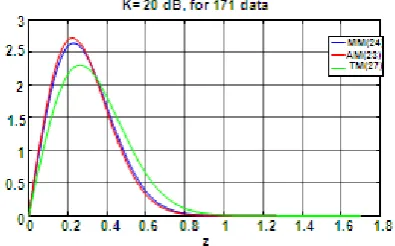
[image:3.595.330.530.253.394.2]Actual, theoretical, and modified Rayleigh Probability Density Functions are plotted according to different K and data values in Fig. 1 through Fig. 6.
Figure 1. Plot of the Actual, Modified, and Theoretical Rayleigh Probability
Density Functions
Figure 2. Plot of the Actual, Modified, and Theoretical Rayleigh Probability Density Functions
[image:3.595.79.277.300.423.2]Figure 3. Plot of the Actual, Modified, and Theoretical Rayleigh Probability Density Functions
[image:3.595.336.525.443.556.2]Figure 4. Plot of the Actual, Modified, and Theoretical Rayleigh Probability Density Functions
Figure 5. Plot of the Actual, Modified, and Theoretical Rayleigh Probability Density Functions
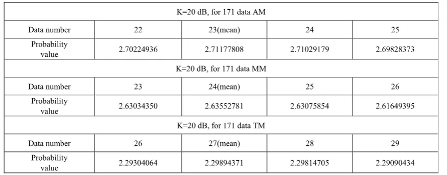
[image:3.595.86.273.461.576.2] [image:3.595.331.529.603.722.2] [image:3.595.89.265.610.728.2]Table 5. The mean values of fz(z),f1z(z), f2z(z) and their values around the means
K=20 dB, for 171 data AM
Data number 22 23(mean) 24 25
Probability
value 2.70224936 2.71177808 2.71029179 2.69828373
K=20 dB, for 171 data MM
Data number 23 24(mean) 25 26
Probability
value 2.63034350 2.63552781 2.63075854 2.61649395
K=20 dB, for 171 data TM
Data number 26 27(mean) 28 29
Probability
value 2.29304064 2.29894371 2.29814705 2.29090434
Table 6. The mean values of fz(z),f1z(z), f2z(z) and their values around the means
K=10 dB, for 171 data AM
Data number 40 41(mean) 42 43
Probability
value 1.52477789 1.52529002 1.52388460 1.52061275
K=10 dB, for 171 data MM
Data number 41 42(mean) 43 44
Probability
value 1.49019207 1.49053635 1.48909413 1.48591223
K=10 dB, for 171 data TM
Data number 47 48(mean) 49 50
Probability
[image:4.595.88.526.97.268.2]value 1.29257103 1.29305214 1.29236036 1.29052165
Table 7. The mean values of fz(z),f1z(z), f2z(z) and their values around the means
K=20 dB, for 1701 data AM
Data number 224 225(mean) 226 227
Probability
value 2.71246757 2.71247918 2.71238249 2.71217797
K=20 dB, for 1701 data MM
Data number 235 236(mean) 237 238
Probability
value 2.57543251 2.57552531 2.57552503 2.57543207
K=20 dB, for 1701 data TM
Data number 264 265(mean) 266 267
Probability
Table 8. The mean values of fz(z),f1z(z), f2z(z) and their values around the means
K=10 dB, for 1701 data AM
Data number 398 399(mean) 400 401
Probability
value 1.52533995 1.52534257 1.52532591 1.52529002
K=10 dB, for 1701 data MM
Data number 417 418(mean) 419 420
Probability
value 1.45500983 1.45501578 1.45500499 1.45497749
K=10 dB, for 1701 data TM
Data number 469 470(mean) 471 472
Probability
value 1.29305056 1.29305723 1.29305214 1.29303533
Table 9. The mean values of fz(z),f1z(z), f2z(z) and their values around the means
K=20 dB, for 17001 data AM
Data number 2236 2237(mean) 2238 2239
Probability
value 2.71248695 2.71248756 2.71248709 2.71248554
K=20 dB, for 17001 data MM
Data number 2361 2362(mean) 2363 2364
Probability
value 2.56916919 2.56916947 2.56916883 2.56916727
K=20 dB, for 17001 data TM
Data number 2638 2639(mean) 2640 2641
Probability
value 2.29941691 2.29941708 2.29941659 2.2994154
Table 10. The mean values of fz(z),f1z(z), f2z(z) and their values around the means
K=10 dB, for 17001 data AM
Data number 3976 3977(mean) 3978 3979
Probability
value 1.52534367 1.52534384 1.52534381 1.52534359
K=10 dB, for 17001 data MM
Data number 4175 4176(mean) 4177 4178
Probability
value 1.45292350 1.45292351 1.45292335 1.45292302
K=10 dB, for 17001 data TM
Data number 4691 4692(mean) 4693 4694
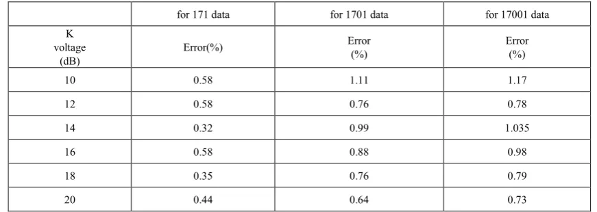
Table 11. Percent errors according to various K and data numbers
for 171 data for 1701 data for 17001 data
K voltage
(dB) Error(%)
Error
(%) Error (%)
10 0.58 1.11 1.17
12 0.58 0.76 0.78
14 0.32 0.99 1.035
16 0.58 0.88 0.98
18 0.35 0.76 0.79
20 0.44 0.64 0.73
For a definite K value if the number of data increases percent error slightly increases as well.
4. Conclusion
In this study, to minimize the difference between the theoretical mean of Rayleigh Probability Density Function and the mean of the plot of Rayleigh function, we modified the equation (10) and obtained the equation (14) as the ultimate expression for the mean.
In actual plots and plots corresponding to theoretical means are shown together.
It is observed from the Table 11 that, for the smaller values of K, percent error increases by the number of data much more than for the larger values of K. For this particular study although the number of data increased 100 times, percent error was just only doubled.
REFERENCES
[1] A. Papoulis. Probability Random Variables and Stochastic Processes, McGraw-Hill, New York, 1965.
[2] J. Goldhirsh, W.J.Vogel. Handbook of Propagation Effects for Vehicular and Personal Mobile Satellite Systems, December, 1998.
[3] D. Lu, K. Yao. Improved Importance Sampling Technique for Efficient Simulation of Digital Communication Systems,IEEE Journal on Select. Areas in Commun.,Vol.6, No.1,67–75, 1988.
[4] W. C. Y. Lee. Mobile Communications Design Fundamentals, H. W. Sams and Co., Indianapolis, Indiana, 1986.
[5] M. Abramowitz, I. Stegun. Handbook of Mathematical Functions, NBS Applies Mathematics Series, Vol.55, U.S. Govt. Printing Office, Washington, DC.,20402,1964. [6] R. H. Clarke. A Statistical Theory of Mobile-Radio
Reception, Bell System Technical Journal, Vol.47, No.6, 329-339,1968.
[7] W. C. Jakes. Microwave Mobile Communications, Wiley, NewYork, 1974.
[8] A. Maaref, S. Aissa. Joint and Marginal Eigen value Distributions of (Non)Central Complex Wishart Matrices and PDF-Based Approach for Characterizing the Capacity Statistics of MIMO Ricean and Rayleigh Fading Channels. Wireless Communications, IEEE Transactions on Vol.6, No.10,3607-3619,2007.
[9] B. Yang, K. B. Letaief, R. S. Chen, Z. Cao. Channel estimation for OFDM transmission in multipath fading channels based on parametric channel modeling, IEEE Trans. Commun., vol.49, 467–478, 2001.
[10] X. Ma, G. B. Giannakis, S. Ohno.Optimal training for block transmissions over doubly-selective wireless fading channels, IEEE Trans.Signal Processing, vol.51, 1351–1366, 2003. [11] G.A. Dimitrakopoulos, C.N. Capsalis. Statistical modeling
of RMS-delay spread under multipath fading conditions in local areas Vehicular Technology, IEEE Transactions on Vol.49, No.5, 1522-1528, 2000.
[12] J. Salo, H.M. El-Sallabi, P. Vainikainen. The distribution of the product of independent Rayleigh random variables. Antennas and Propagation, IEEE TransactionsVol.54,No.2, 639-643, 2006.
[13] B. Rivet, L. Girin,C. Jutten. Log-Rayleigh Distribution: A Simple and Efficient Statistical Representation of Log-Spectral Coefficients Audio, Speech, and Language Processing, IEEE Transactions on Vol.15, No.3, 796-802,2007.
[14] C.Yunxia, C. Tellambura. Joint distribution functions of three or four correlated Rayleigh signals and their application in diversity system analysis. Global Telecommunications Conference. Vol.5, 3368-3372, 2004. [15] D.A.Abraham, A.P.Lyons. Exponential scattering and
K-distributed reverberation. OCEANS,MTS/IEEE Conference and ExhibitionVol.3, 1622-1628,2001.
[16] P.M. Shankar. Outage probabilities in shadowed fading channels using a compound statistical model, Communications, IEE ProceedingsVol.152, No.6, 828-832, 2005.
[18] J. Lei, Y. Tan. Geometrically Based Statistical Channel Models for Outdoor and Indoor Propagation Environments Vehicular Technology, IEEE Transactions on Vol.56, No.6, 3587-3593, 2007.
[19] H.Lu,Y.Chen,N. Cao. Accurate Approximation to the PDF of the Product of Independent Rayleigh Random Variables Antennas and Wireless Propagation Letters, IEEE Vol.10, 1019-1022, 2011.
[20] D.Wong, D.C. Cox. Estimating local mean signal power level in a Rayleigh fading environment, Vehicular Technology, IEEE Transactions on Vol.48, No.3, 956-959, 1999.
[21] R. Narasimhan, D.C. Cox.Mean and variance of the local maxima of a Rayleigh fading envelope, Communications Letters, IEEE Vol.4, No.11, 352-353, 2000.
[22] C. Gao, M. Zhao, S. Zhou, Yan Yao.A new calculation on the mean capacity of MIMO systems over Rayleigh fading channels, Personal, Indoor and Mobile Radio Communications, 14th IEEE Proceedings, Vol.3, 2267–2270, 2003.