Program for Using Path Profile and Coordinate Geometry Approach in the Determination of the Exact Radius of Curvature for Rounded Edge Diffraction Loss Computation

(1)

Program for Using Path Profile and Coordinate

Geometry Approach in the Determination of

the Exact Radius of Curvature for Rounded

Edge Diffraction Loss Computation

Kalu Constance

Department of Electrical/ Electronic and Computer Engineering, University of Uyo, Nigeria

Abstract In this paper, the design of a program

algorithm for using path profile and coordinate geometry approach in the determination of the exact radius of curvature for rounded edge diffraction loss computation is presented. In addition to the radius of curvature, the program determined the values of other essential parameters required for the computation of rounded edge diffraction loss. The additional parameters include; occultation distance, the line of sight clearance height and the external angle between the tangent lines to the path profile. Importantly, the requisite mathematical expressions and detailed algorithm for the program are presented. Then a program was developed in Visual Basic for Application (VBA) based on the algorithm. Furthermore, sample elevation data was used to demonstrate the effectiveness of the program in the determination of the radius of curvature along with the other essential parameters required for the rounded edge diffraction loss computation. A sample path elevation profile was obtained using Geocontext path profile software for a 5233.692 m path that has a hilly obstruction with a maximum elevation of 593.0363 m that occurred at about a distance of 1861.649 m from the transmitter. The program result showed that for the sample path profile the rounded edge should be of a circle with a radius of 9,392.78 m, the occultation distance is 2,002.15 m, the line of sight clearance height which is 176.469 m and finally the angle between the tangent lines at their point of intersection is 0.212916 radians. The result is particularly useful because it is easy to generate the coordinates of elevation points which the program developed in this paper can use to automatically generate the essential parameters needed for the computation of rounded edge diffraction loss.

Keywords Diffraction, Diffraction Loss, Plane

Geometry, Radius of Curvature, Rounded Edge

Diffraction

1. Introduction

In wireless communication systems, diffraction loss caused by obstructions in the signal depends on the nature of the obstruction [1, 2, 3, 4, 5, 6]. Consequently, among other things, the approach used to determine diffraction loss depends on the location and dimensions of the obstruction in respect of the signal that is being considered [7, 8, 9, 10, 11, 12, 13, 14]. Particularly, rounded edge diffraction model is used to determine the diffraction loss that can be caused by isolated hilly obstructions along the wireless signal path [15, 16, 17]. The rounded edge method of diffraction loss requires the determination of the radius of curvature of the circle to be fitted to the vicinity of the hilly obstruction apex. Although some approximate methods exists for estimation of an approximate value of the radius of the circle expected for the rounded edge [15, 17, 18, 19, 20], however, through the use of plane geometry an exact radius of curvature can be determined for any given hilly or plateau obstruction.

(2)

obstruction apex.

However, the program presented in this paper can be used to read in the longitude, latitude and elevation of each data point provided in the elevation profile dataset and then use the Haversine formula to determine the distance from the transmitter to each of the longitude and latitude. Then based on plane geometry principles, relevant mathematical expressions are presented and used to determine the exact radius of curvature for the rounded edge diffraction loss computation. The requisite algorithms for the program are presented along with sample numerical example to demonstrate how the program can be used.

2. The Algorithm for the Program to

Determine the Exact Radius of

Curvature

The task to be handled by the algorithm is decomposed into seven (7) major steps, namely;

STEP 1: Obtain the path elevation profile data from the transmitter to the receiver including the obstruction elevation profile in the path.

STEP 2: Determine the path length and distance between the transmitter and each of the elevation data samples

STEP 3: Determine the Maximum Elevation Parameters STEP 4: Determination of the tangent point A from the transmitter

STEP 5: Determination of the tangent point B from the receiver

STEP 6: Determination of the radius of curvature of the rounded edge

STEP 7: Determination of the occultation distance and the angles 𝛼 and 𝛽

Within each of the major steps are sub-steps. The details of each major step are then presented along with their accompanying mathematical expressions and algorithms.

STEP 1: Obtain the path elevation profile data from the transmitter to the receiver including the obstruction elevation profile in the path.

The path elevation profile often includes the geo-coordinate (longitude and latitude) of data points along with the elevation at each of the geo-coordinates from the transmitter to the receiver. Assuming there are N elevation data point samples captured in the path and the transmitter location is taken as the starting point with data point sampling number n = 1 then the receiver has n = N.

The raw elevation profile data will contain at least the geo-coordinate (longitude and latitude) given as𝐿𝐴𝑇𝐷_𝑛,

𝐿𝑂𝑁𝐺𝐷𝑛 along with the elevation (𝐸𝑛) at each of the

geo-coordinate points, where n = 1, 2,…, N.

STEP 1.1 INPUT N // Input the number of elevation profile data points expected in the data set

STEP 1.2 FOR n = 1 TO N STEP 1 STEP 1.3 INPUT 𝐿𝐴𝑇𝐷_𝑛

STEP 1.4 INPUT 𝐿𝑂𝑁𝐺𝐷_𝑛 STEP 1.5 INPUT 𝐸_𝑛 STEP 1.6 NEXT n

STEP 2: Determine the path length and distance between the transmitter and each of the elevation data samples

When the longitude and latitude of data points are given, then the Haversine formula can be used to determine the distance, 𝒅_𝒏 in Km between the transmitter and each of the elevation data point n as follows as:

𝑑𝑛 =

2(𝑅)

⎩ ⎨ ⎧

� sin�

𝐿𝐴𝑇𝑛−𝐿𝐴𝑇1

2 �

2

+

((cos(𝐿𝐴𝑇1))cos(𝐿𝐴𝑇𝑛)) sin�𝐿𝑂𝑁𝐺𝑛−𝐿𝑂𝑁𝐺₂ 1� 2

2

⎭ ⎬ ⎫

(1) where 𝐿𝐴𝑇₁, 𝐿𝐴𝑇_𝑛 , 𝐿𝑂𝑁𝐺₁ and 𝐿𝑂𝑁𝐺_𝑛 are all in Radians whereas 𝐿𝐴𝑇𝐷_𝑛 is the latitude in degrees and

𝐿𝑂𝑁𝐺𝐷𝑛 is 𝑡ℎ𝑒 longitue in degrees. Hence,

𝐿𝐴𝑇𝑛 = (𝐿𝐴𝑇𝐷𝑛₁₈₀ ∗3.142) (2) 𝐿𝑂𝑁𝐺𝑛 = (𝐿𝑂𝑁𝐺𝐷₁₈₀𝑛 ∗3.142) (3)

Where

𝐿𝐴𝑇1 and 𝐿𝐴𝑇𝑛 are the latitude of the coordinates of

point1 (the transmitter) and point n respectively).

𝐿𝑂𝑁𝐺1 and 𝐿𝑂𝑁𝐺𝑛 are the longitude of the

coordinates of point1 (the transmitter) and point n respectively.

R = radius of the earth = 6371 km

R varies from 6356.752km at the poles to 6378.137 km at the equator

When n = N, then 𝑑_𝑛 =𝑑_𝑁 =𝑑 which is the path length or the distance between the transmitter and the receiver.

STEP 2.1 𝐿𝐴𝑇₁ = (𝐿𝐴𝑇𝐷𝑛 ∗3.142)

180

STEP 2.2 𝐿𝑂𝑁𝐺₁ = (𝐿𝑂𝑁𝐺𝐷₁₈₀𝑛 ∗3.142) STEP 2.3 𝑑_𝑛 = 0

STEP 2.4 FOR n = 2 TO N STEP 1 STEP 2.5 𝐿𝐴𝑇_𝑛 = (𝐿𝐴𝑇𝐷𝑛 ∗3.142)

180

STEP 2.6 𝐿𝑂𝑁𝐺_𝑛 = (LONG inDegrees ∗3.142)

180

STEP 2.7 𝑑_𝑛 = 2(𝑅) ��sin�𝐿𝐴𝑇𝑛−𝐿𝐴𝑇1

2 �

2

+ ((cos(𝐿𝐴𝑇1))cos(𝐿𝐴𝑇𝑛)) sin�𝐿𝑂𝑁𝐺𝑛−𝐿𝑂𝑁𝐺₂ 1� 2

2

(3)

STEP 3: Determine the Maximum Elevation Parameters

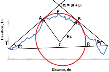
In order to determine the radius of curvature for rounded edge diffraction loss some key parameters are required and they are determined from the path elevation profile data as shown in Figure 1 and in Figure 2. Figure 1 shows a typical elevation profile plot with a hill obstruction between the transmitter (T) and the receiver (R) and the obstruction (hill) has maximum elevation at point P. The maximum elevation parameters needed are the maximum elevation,

𝐸𝑛𝑚𝑎𝑥 and the distance, 𝑑𝑛𝑚𝑎𝑥of the maximum elevation

point from the transmitter.

Figure 1. A typical elevation profile plot showing the maximum elevation point P

Figure 2. A typical elevation profile plot showing the key points of interest needed in the determination of the radius of curvature for rounded edge diffraction loss

Based on the N elevation profile data, the maximum elevation parameters are determined as follows;

STEP 3.1 nmax = 1 // Initialise the data point number for the maximum elevation point, P

STEP 3.2 𝑑_{𝑛𝑚𝑎𝑥} = 𝑑₁ // Initialise the distance of the maximum elevation at point, P

STEP 3.3 𝐸_{𝑛𝑚𝑎𝑥} = 𝐸₁ // Initialise the maximum elevation at point, P

STEP 3.4 FOR n = 2 TO N STEP 1

STEP 3.5 IF ( 𝐸_𝑛>𝐸_{𝑛𝑚𝑎𝑥} THEN (nmax = n ; 𝐸𝑛𝑚𝑎𝑥 = 𝐸𝑛; 𝑑𝑛𝑚𝑎𝑥 = 𝑑𝑛 ) ENDIF

STEP 3.6 NEXT n

STEP 4: Determination of the tangent point A from the transmitter

The slope, 𝑚𝑡_𝑛of the line from the transmitter, (with coordinates 𝑑₁,𝐸₁) to the elevation points n =2, 3,…, nmax (with coordinates 𝑑_𝑛,𝐸_𝑛) are computed one at a time. The point A (in Figure 2) with the maximum absolute value of𝑚𝑡_𝑛, (that is, maximum|𝑚𝑡_𝑛|) is the tangent point for the line from the transmitter to the elevation profile. Now, 𝑚𝑡_𝑛 is given as;

𝑚𝑡𝑛=𝐸_𝑑𝑛_𝑛−𝐸_−𝑑1₁ (4)

STEP 4.1 ntmax = 1 // Initialise the data point number for the maximum absolute value of slope for elevation points between T and P

STEP 4.2 mt_ntmax = 0 // the maximum absolute value of slope for elevation points between T and P

STEP 4.3 𝐸𝑡_ntmax = 𝐸₁ // Initialise the elevation with the maximum absolute value of slope for elevation points between T and P

STEP 4.3 FOR n = 2 TO nmax STEP 1

STEP 4.4 𝑑𝑡_ntmax = 𝑑₁ // Initialise the distance with the maximum absolute value of slope for elevation points between T and P

STEP 4.5 FOR n = 2 TO nmax STEP 1 STEP 4.6 𝑚𝑡_𝑛=𝐸_𝑑𝑛−𝐸1

𝑛−𝑑1

STEP 4.7 IF (|𝑚𝑡_𝑛| > |𝑚𝑡_ntmax| THEN (ntmax = n ; 𝑚𝑡ntmax=𝑚𝑡𝑛; 𝐸𝑡ntmax=𝐸𝑛; 𝑑𝑡ntmax=

𝑑𝑛 ) ENDIF

STEP 4.8 NEXT n

STEP 5: Determination of the tangent point B from the receiver

The slope, 𝑚𝑟_𝑛of the line from the receiver, (with coordinates 𝑑_𝑁,𝐸_𝑁) to the elevation points n = N-1, N-2, N-3,…, N-nmax (with coordinates 𝑑_𝑛,𝐸_𝑛) are computed one at a time . The point B (in Figure 2) with the maximum absolute value of 𝑚𝑟_𝑛, (that is maximum |𝑚𝑟_𝑛|) is the tangent point for the line from the receiver to the elevation profile. Now, 𝑚𝑟_𝑛 is given as;

𝑚𝑟𝑛=𝐸_𝑑𝑛_𝑛−𝐸_−𝑑𝑁_𝑁 (5)

STEP 5.1 nrmax = 1 // Initialise the data point number for the maximum absolute value of slope for elevation points between P and R

STEP 5.2 𝐦𝐫_{𝐧𝐫𝐦𝐚𝐱} = 𝟎 // the maximum absolute value of slope for elevation points between P and R

STEP 5.3 𝐸𝑟_nrmax = 𝐸_N // Initialise the elevation with the maximum absolute value of slope for elevation points between P and R

[image:3.595.62.288.234.348.2] [image:3.595.64.288.385.534.2]

(4)

STEP 5.5 FOR n = N TO nmax STEP -1 STEP 5.6 𝑚𝑟_𝑛=𝐸𝑛−𝐸𝑁

𝑑𝑛−𝑑𝑁

STEP 5.7 IF (|𝑚𝑟_𝑛| > |𝑚𝑟_nrmax| THEN (nrmax = n ; 𝑚𝑟nrmax=𝑚𝑟𝑛; 𝐸𝑟nrmax=𝐸𝑛; 𝑑𝑟nrmax=

𝑑𝑛 ) ENDIF

STEP 5.8 NEXT n

STEP 6: Determination of the radius of curvature of the rounded edge

As Shown in Figure 2, the required circle has its centre at point C with coordinates d_C and E_C.The slope of line TA from the transmitter, T to the tangent point A has been found in STEP 4 as 𝑚𝑡_ntmax while the slope of line RB from the receiver, R to the tangent point B has been found in STEP 5 as 𝑚𝑟_nrmax. Now, the circle radius, AC is perpendicular to line TA at point A so the slope of line AC is − � 1

mtntmax�. Similarly, the slope of line BC is

− �_mr 1

nrmax.� . The coordinates of C, which is the

intersection point of line AC and line BC is found by coordinate geometry approach to be;

dC= �

�_mrnrmaxdB �−�_mtntmaxdA �+(EB−EA)

��_mrnrmax1 �−�_mtntmax1 �� (6)

EC =

= EB−_mr_nrmax1 ��

�_mrnrmaxdB �−�_mtntmaxdA �+(EB−EA)

��_mrnrmax1 �−�_mtntmax1 �� −dB�(7)

Finally, the circle radius, BC which is denoted as 𝑅_𝐶in Figure 2 is given as ;

𝑅𝐶 = 2�((dB−dC)2 + (EB−EC)2) (8)

STEP 6.1 E_A=𝐸𝑡_ntmax STEP 6.2 d_A= 𝑑𝑡_ntmax STEP 6.3 E_B=𝐸𝑟_nrmax STEP 6.4 d_B=𝑑𝑟_nrmax STEP 6.5 d_C= ��

dB

mrnrmax�−�mtntmaxdA �+(EB−EA)

��_mrnrmax1 �−�_mtntmax1 ��

STEP 6.6 EC =

= EB−_mr1 nrmax ⎝ ⎜ ⎛ ⎣ ⎢ ⎢ ⎢ ⎡� dB

mrnrmax�− �

dA

mtntmax� + (EB−EA)

��_mr1

nrmax�− �

1

mtntmax�� _⎦⎥

⎥ ⎥ ⎤

−dB

⎠ ⎟ ⎞

STEP 6.7 𝑅_𝐶 = 2�((d_B−d_C)2 + (E_B−E_C)2)

STEP 7: Determination of the occultation distance and the angles 𝛂𝛂 and 𝛃𝛃

The occultation distance, D_OC is given as;

DOC= |dB−dA| (9)

The slope, 𝑚𝑡𝑟of the line from the transmitter, n=1 to the receiver, n=N is given as;

𝑚𝑡𝑟=𝐸𝑁−𝐸1

𝑑𝑁−𝑑1 (10)

Already, the slope of the line RB is mr_nrmaxand the slope of the line TA is mt_ntmax, then angle 𝛼 and angle 𝛽 in radians are given as ;

𝛼𝛽𝑟= (mrnrmax−𝑚𝑡𝑟)

�1+mrnrmax(𝑚𝑡𝑟)� (11)

𝛽𝑡= (𝑚𝑡𝑟−mtntmax)

�1+𝑚𝑡𝑟(mtntmax)� (12)

𝛼=𝛽𝑡+𝛽𝑟 (13) The equation of the line TR from the transmitter, n=1 to the receiver, n=N with slope𝑚𝑡𝑟, is given as;

𝑚𝑡𝑟(dn)− En−(𝑚𝑡𝑟(dN)−EN) = 0 (14)

The distance from apex P point with coordinates (d_p, E_p) to the line m(d_n)−E_n−(m(d_N)−E_N) = 0 is denoted as h where h is the clearance height which is given as:

ℎ= �𝑚𝑡𝑟�dp�−Ep−(𝑚𝑡𝑟(dN)−EN)�

�(12₋₍_𝑚𝑡𝑟₎2₎

2 (15)

STEP 7.1 D_OC= |d_B−d_A| STEP 7.2 𝛽𝑟= (mrnrmax−𝑚𝑡𝑟)

�1+mrnrmax(𝑚𝑡𝑟)�

STEP 7.3 𝛽𝑡= (𝑚𝑡𝑟−mtntmax)

�1+𝑚𝑡𝑟(mtntmax)�

STEP 7.4 𝛼=𝛽𝑡+𝛽𝑟

STEP 7.5 ℎ= �𝑚𝑡𝑟�dp�−Ep−(𝑚𝑡𝑟(dN)−EN)�

�(12₋₍_𝑚𝑡𝑟₎2₎ 2

3. The Program Implementation,

Numerical Example and Discussion

of Result

(5)

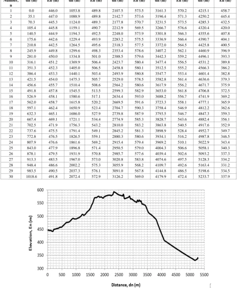
Table 1. The 511 elevation profile data of the sample path

n =1 to n = 30 n =31 to n = 60 n =61 to n = 90 n =91 to n = 120 n =121 to n = 150 Data

Sample Number,

n

Distance, dn (m)

Elevation, En (m)

1 0.0 446.0 1053.8 489.8 2107.5 573.5 3161.3 570.2 4215.1 458.7

2 35.1 447.0 1088.9 489.8 2142.7 573.6 3196.4 571.3 4250.2 445.4

3 70.3 445.3 1124.0 489.3 2177.8 570.7 3231.5 573.5 4285.3 432.5

4 105.4 445.8 1159.1 490.7 2212.9 569.5 3266.7 576.6 4320.4 420.0

5 140.5 444.9 1194.3 492.5 2248.0 573.9 3301.8 566.3 4355.6 407.8

6 175.6 442.6 1229.4 493.9 2283.2 575.5 3336.9 566.4 4390.7 404.1

7 210.8 442.5 1264.5 495.6 2318.3 577.5 3372.0 564.5 4425.8 400.5

8 245.9 449.8 1299.6 498.3 2353.4 578.6 3407.2 562.1 4460.9 396.9

9 281.0 450.0 1334.8 501.0 2388.5 579.6 3442.3 559.2 4496.1 393.3

10 316.1 451.2 1369.9 506.4 2423.7 580.4 3477.4 556.5 4531.2 389.8

11 351.3 452.3 1405.0 506.5 2458.8 580.1 3512.5 555.2 4566.3 386.2

12 386.4 453.3 1440.1 503.4 2493.9 580.8 3547.7 553.4 4601.4 382.8

13 421.5 454.0 1475.3 505.7 2529.0 578.5 3582.8 561.4 4636.6 379.3

14 456.6 455.7 1510.4 508.6 2564.2 580.6 3617.9 556.2 4671.7 375.9

15 491.8 457.8 1545.5 513.5 2599.3 582.9 3653.0 561.8 4706.8 372.5

16 526.9 458.1 1580.6 517.1 2634.4 593.0 3688.2 556.7 4741.9 369.2

17 562.0 458.7 1615.8 520.2 2669.5 591.6 3723.3 558.1 4777.1 365.9

18 597.1 462.4 1650.9 523.4 2704.7 590.3 3758.4 546.9 4812.2 362.6

19 632.3 465.1 1686.0 527.9 2739.8 587.9 3793.5 546.7 4847.3 359.3

20 667.4 469.1 1721.1 534.4 2774.9 585.3 3828.7 543.6 4882.4 356.1

21 702.5 471.9 1756.3 543.2 2810.0 583.2 3863.8 540.5 4917.6 352.9

22 737.6 475.5 1791.4 549.1 2845.2 581.3 3898.9 528.4 4952.7 349.7

23 772.8 476.5 1826.5 559.1 2880.3 580.6 3934.1 516.2 4987.8 346.5

24 807.9 476.6 1861.6 569.2 2915.4 579.4 3969.2 510.1 5022.9 343.4

25 843.0 477.9 1896.8 571.4 2950.5 579.0 4004.3 506.6 5058.1 340.3

26 878.1 479.5 1931.9 570.8 2985.7 577.6 4039.4 502.6 5093.2 337.3

27 913.3 483.5 1967.0 573.0 3020.8 583.8 4074.6 497.5 5128.3 334.2

28 948.4 486.6 2002.2 575.3 3055.9 568.2 4109.7 492.6 5163.4 331.2

29 983.5 490.5 2037.3 576.1 3091.0 567.8 4144.8 486.5 5198.6 334.5

30 1018.6 491.8 2072.4 572.9 3126.2 569.0 4179.9 472.4 5233.7 337.9

[image:5.595.57.540.99.741.2]

[image:5.595.57.538.136.720.2]

(6)

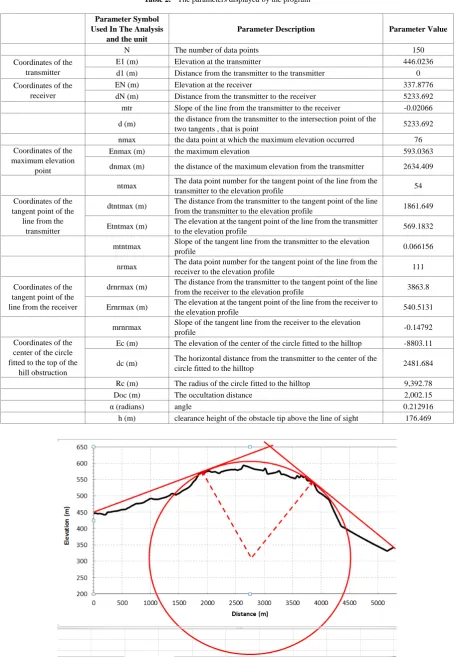
Table 2. The parameters displayed by the program

Parameter Symbol Used In The Analysis

and the unit

Parameter Description Parameter Value

N The number of data points 150

Coordinates of the transmitter

E1 (m) Elevation at the transmitter 446.0236

d1 (m) Distance from the transmitter to the transmitter 0

Coordinates of the receiver

EN (m) Elevation at the receiver 337.8776

dN (m) Distance from the transmitter to the receiver 5233.692

mtr Slope of the line from the transmitter to the receiver -0.02066

d (m) the distance from the transmitter to the intersection point of the

two tangents , that is point 5233.692

nmax the data point at which the maximum elevation occurred 76

Coordinates of the maximum elevation

point

Enmax (m) the maximum elevation 593.0363

dnmax (m) the distance of the maximum elevation from the transmitter 2634.409

ntmax The data point number for the tangent point of the line from the

transmitter to the elevation profile 54

Coordinates of the tangent point of the

line from the transmitter

dtntmax (m) The distance from the transmitter to the tangent point of the line

from the transmitter to the elevation profile 1861.649

Etntmax (m) The elevation at the tangent point of the line from the transmitter

to the elevation profile 569.1832

mtntmax Slope of the tangent line from the transmitter to the elevation

profile 0.066156

nrmax The data point number for the tangent point of the line from the

receiver to the elevation profile 111

Coordinates of the tangent point of the line from the receiver

drnrmax (m) The distance from the transmitter to the tangent point of the line

from the receiver to the elevation profile 3863.8

Ernrmax (m) The elevation at the tangent point of the line from the receiver to

the elevation profile 540.5131

mrnrmax Slope of the tangent line from the receiver to the elevation

profile -0.14792

Coordinates of the center of the circle fitted to the top of the

hill obstruction

Ec (m) The elevation of the center of the circle fitted to the hilltop -8803.11

dc (m) The horizontal distance from the transmitter to the center of the

circle fitted to the hilltop 2481.684

Rc (m) The radius of the circle fitted to the hilltop 9,392.78

Doc (m) The occultation distance 2,002.15

α (radians) angle 0.212916

h (m) clearance height of the obstacle tip above the line of sight 176.469

[image:6.595.70.527.84.744.2]

(7)

The program result showed that the 5233.692 m path has a hilly obstruction with a maximum elevation of 593.0363 m that occurred at about a distance of 1861.649 m from the transmitter. In order to use rounded edge diffraction method to determine the diffraction loss the hilly obstruction will present to signals along that path, a rounded edge or circle with a radius of 9,392.78 m should be fitted to the top of the hilly obstruction. Other required parameters for the rounded edge diffraction loss computation are the occultation distance which 2,002.15 m, the line of sight clearance height which is 176.469 m and finally, the angle, α between the tangent lines at their point of intersection which is 0.212916 radians.

Advantage of the approach presented in this paper: The method presented in this paper gives the exact radius of curvature of the circle fitted to the vicinity of the hill (obstruction) apex whereas the conventional methods used to determine the radius of the circle are approximates methods which can be found in [18,20 ]. Moreover, the computer program-based approach makes it easier to automatically determine the exact radius of curvature once the elevation profile data that consist of the longitude, the latitude and the elevation of the points along the signal path are known. Fortunately, the elevation profile data are readily generated using online elevation profile software. Essentially, this paper enables the user to take advantage of available technology to simplify the process of determining the exact radius of curvature for rounded edge diffraction loss computation.

4. Conclusions

The coordinate geometry approach that uses path profile to determine the exact radius of curvature for rounded edge diffraction loss is presentation is presented. The requisite mathematical expressions and detailed algorithm are presented. Then a program was developed in Visual Basic for Application (VBA) based on the algorithm. Furthermore, sample elevation data was used to demonstrate the effectiveness of the program in the determination of the radius of curvature along with the other essential parameters required for the rounded edge diffraction loss computation.

REFERENCES

[1] Abdulrasool, A. S., Aziz, J. S., & Abou-Loukh, S. J. (2017). Calculation Algorithm for Diffraction Losses of Multiple Obstacles Based on Epstein–Peterson Approach. International Journal of Antennas and Propagation, 2017.

[2] Rappaport, T. S., MacCartney, G. R., Sun, S., Yan, H., & Deng, S. (2017). Small-scale, local area and transitional millimeter wave propagation for 5G communications. IEEE Transactions on Antennas and Propagation, 65(12),

6474-6490.

[3] Loo, Z. B., Chong, P. K., Lee, K. Y., & Yap, W. S. (2017). Improved path loss simulation incorporating three-dimensional terrain model using parallel coprocessors. Wireless Communications and Mobile Computing, 2017.

[4] Amorim, R., Mogensen, P., Sorensen, T., Kovács, I. Z., & Wigard, J. (2017, June). Pathloss measurements and modeling for UAVs connected to cellular networks. In Vehicular Technology Conference (VTC Spring), 2017 IEEE 85th (pp. 1-6). IEEE.

[5] Blaunstein, N., Censor, D., Katz, D., Freedman, A., & Matityahu, I. (2003). Radio propagation in rural residential areas with vegetation. Progress in Electromagnetics Research, 40, 131-153.

[6] Pélet, E. R., Salt, E. J., & Wells, G. (2004, May). Signal distortion caused by tree foliage in a 2.5 GHz channel. In Canadian Conference on Electrical and Computer Engineering 2004 (IEEE Cat. No. 04CH37513) (Vol. 3, pp. 1449-1452). IEEE.

[7] Kapusuz, K. Y., & Kara, A. (2014). Determination of scattering center of multipath signals using geometric optics and Fresnel zone concepts. Engineering Science and Technology, an International Journal, 17(2), 50-57.

[8] Kukshya, V. (2001). Wideband Terrestrial Path Loss Measurement Results for Characterization of Pico-cell Radio Links at 38 GHz and 60 GHz Bands of Frequencies (Doctoral dissertation, Virginia Tech).

[9] Helhel, S., Ozen, S., & Göksu, H. (2008). Investigations of GSM signal variation depending weather conditions. Progress in Electromagnetics Research, 1, 147-157.

[10]Simunek, M., Pechac, P., & Fontan, F. P. (2011). Excess loss model for low elevation links in urban areas for UAVs. Radioengineering, 20(3), 561-568.

[11]Ballot, M. (2014). Radio-wave propagation prediction model tuning of land cover effects. IEEE Transactions on Vehicular Technology, 63(8), 3490-3498.

[12]Meng, Y. S., & Lee, Y. H. (2010). Investigations of foliage effect on modern wireless communication systems: A review. Progress in Electromagnetics Research, 105, 313-332.

[13]Neskovic, A., Neskovic, N., & Paunovic, G. (2000). Modern approaches in modeling of mobile radio systems propagation environment. IEEE Communications Surveys & Tutorials, 3(3), 2-12.

[14]Spencer, T. A. (2006). Inverse diffraction propagation applied to the parabolic wave equation model for geolocation applications (Doctoral dissertation, Queensland University of Technology).

[15]Chikezie, A., Uko, M. C., & Nwokonko, S. C. (2017). Comparative Analysis of the Impact of Frequency on the Radius of Curvature of Single and Double Rounded Edge Hill Obstruction. Mathematical and Software Engineering, 3(2), 164-172.

(8)

WRIGHT-PATTERSON AFB OH SCHOOL OF ENGINEERING AND MANAGEMENT.

[17]Uko M. C., Onwuzuruike V. K., Eke G. K. (2017) Comparative Study of Radius of Curvature of Rounded Edge Hill Obstruction Based on Occultation Distance and ITU-R 526-13 Methods. American Journal of Software Engineering and Applications; 6(3): 74-79

[18]Seybold, J. S. (2005). Introduction to RF propagation. John Wiley & Sons.

[19]International Telecommunication Union, “Recommendation ITU-R P. 526-13: “Propagation by diffraction”, Geneva, 2013.

[20]Barué, G. (2008). Microwave engineering: land & space