A chaotic quantum bee colony optimization for thinned array

Journal of Chemical and Pharmaceutical Research, 2014, 6(7):685-694

Research Article

_{CODEN(USA) : JCPRC5}

ISSN : 0975-7384

A chaotic quantum bee colony optimization for thinned array

Hongyuan Gao* and Yanan Du

College of Information and Communication Engineering, Harbin Engineering University, Harbin, China

_____________________________________________________________________________________________

ABSTRACT

Design a new novel intelligence algorithm which is called as chaotic quantum bee colony optimization (CQBCO) for discrete optimization problem. The proposed CQBCO applies the chaotic theory to quantum bee colony optimization (QBCO), which is an effective discrete optimization algorithm. Then the proposed chaotic quantum bee colony algorithm is used to solve benchmark functions and optimization problem of thinned array. By hybridizing the quantum bee colony optimization and quantum computing theory, the quantum state and binary state of the bees can be well evolved by simulated quantum rotation gate and chaotic mechanical. The new thinned array method based on CQBCO can search the global optimal solution. Simulation results for thinned array are provided to show that the proposed thinned array method is superior to the thinned array methods based on other three intelligence algorithms.

Key words: Quantum bee colony optimization, thinned array, chaotic, particle swarm optimization

_____________________________________________________________________________________________

INTRODUCTION

As we all know that natural system is one of the affluent sources of inspiration for designing new intelligent algorithms. For intelligence algorithms are important scientific domains that are closely related to biological phenomenon existing in nature, some algorithms such as particle swarm optimization (PSO) [1-2] and bee colony optimization [3] are widely studied for all kinds of applications . At present, particle swarm optimization [4] and bee colony optimization [5] were widely used to solve engineering optimization problem, but the global convergent performance should be improved.

In order to improve classic intelligent algorithm, the quantum computing theory is introduced into conventional intelligence algorithm and a better performance is obtained [6]. Quantum-inspired genetic algorithm (QGA) which is a promising genetic algorithm developing in recent years, and it is the product of merging quantum computing theory with genetic algorithm. In QGA, quantum bit encoding represents the chromosome, and evolutionary process of chromosomes is implemented by using quantum rotation gate. Now, we pay more attention to quantum optimization algorithm because it has a strong ability for global search with small population size, rapid convergence and short computing time [7]. Based on quantum computing and bee colony optimization, quantum bee colony optimization (QBCO) is proposed as an effective swarm intelligence algorithm [8]. The results of simulation comparisons show that the performance of the QBCO algorithm is competitive to other intelligence computing algorithms with an advantage of using fewer control parameters.

______________________________________________________________________________

A low side lobe amplitude taper is generated by strategically positioning equally weighted elements in aperiodic arrays domain. Deriving the element positions to obtain a perfect side lobe level by using simple analytical methods are not available [9]. Instead, merge the element density with a region of the array to the amplitude density of the low side lobe amplitude taper for the same size aperture is used for most aperiodic array synthesis methods [10]. The element density at the center of the array is greatest and gradually decreases to the edges. As a rule, side lobes close to the main beam decrease but those far from the main beam increase [11] (which is usually quite acceptable). Aperiodic array synthesis methods target a maximum relative side lobe level by using a given probability [12].

Thinning array for low side lobes includes inspecting a rather large number of possibilities in order to find the best thinned aperture. It is only practical for small arrays if checking of all possible element combinations [13]. Most optimization methods are not well suited for thinning arrays such as down-hill simplex, Powell’s method, and conjugate gradient. Those methods can only optimize a few continuous variables and drop into local minima easily [14]. Those methods developed for continuous parameters, but the array thinning problem involves discrete parameters. Although dynamic programming can optimize a large parameter set, it is easily effect by local solutions [15].

As we all know genetic algorithms [16] and simulated annealing algorithm [17] are suited for thinning arrays because they do not limit to the number of variables of optimization. Although these algorithms can handle very large arrays, they are quite slow to find the optimal structure of thinned array. In order to achieve more robust and efficient performances for thinned array, CQBCO is proposed to design optimal structure of thinned array.

CHAOTIC QUANTUM BEE COLONY OPTIMIZATION

In order to deal with discrete optimization problems by using chaotic mechanic and quantum bee colony theory, CQBCO is designed. The quantum evolutionary algorithms use quantum coding, called on a quantum bit [18], for the probabilistic representation that is based on the concept of quantum bit, and a quantum position is defined as a string of quantum bits. The quantum position of the ith bee is defined as

1 2

1 2

i i iD

i

i i iD

v

v

v

β

β

β





=









L

L

q

(1)

where

|

v

id

|

2

+

|

β

id

|

2

=

1

,

(

d

=

1, 2,

L

,

D

)

. In CQBCO,

v

id and

β

id are defined as real numbers and

0

≤

v

_id

≤

1

,

0

≤

β

_id

≤

1

[8].

The evolutionary process of quantum bee colony is mainly completed through the update of quantum position. The update of quantum position is obtained by quantum rotation gate. Quantum rotation gate can be described by equation

(2). If the quantum rotation angle is

ϕ

_idt+1, a quantum bit position t

[

t

,

t

]

T

id

=

v

id

β

id

q

is updated by using the rotation

gate

(

ϕ

idt 1

)

+

U

. The dth quantum bit position

q

t_idof the ith quantum position is updated as

1 1

1 1

1 1

cos

sin

abs( (

)

)

abs(

)

sin

cos

t t

id id

t t t t

id id id _{t t} id

id id

ϕ

ϕ

ϕ

ϕ

ϕ

+ +

+ +

+ +



₋



=

=













q

U

q

q

(2)

where

abs()

is an absolute value function which makes quantum bit in the real domain [0,1].

To reduce computation of CQBCO, we use a series simple quantum bits to represent position of bee in CQBCO. A

quantum position of the ith bee is simplified as

v

ti

=

(

v v

it₁

,

it₂

,

L

,

v

iDt

)

where quantum bit is limited to

0

1

t id

v

≤

≤

,

1, 2,

,

d

=

L

D

.

Chaotic quantum bee colony optimization is a novel optimization algorithm inspired by social behavior metaphor of bees. Each bee, flies in a D-dimensional space according to the historical experiences of its own and its colleagues. In CQBCO, the bee colony contains two groups of bees: employed bees and onlookers. First half of the quantum bee colony consists of the employed bees and the second half includes the onlookers.

1 2

(

,

,

,

)

t t t t

i

=

x

i

x

i

L

x

iD

x

,

(

i

=

1, 2,

L

, )

h

, which is a latent solution of optimization problem. The ith bee’s quantum position is

v

t_i

=

(

v v

_it₁

,

_it₂

,

L

,

v

_iDt

)

,

(

i

=

1, 2,

L

, )

h

which is measured and produced food source’s position. Employed bees and onlookers learn different food source information from bee colony. Until now the optimal position

of the

i

th

bee is expressed as

p

it

=

(

p

it₁

,

p

it₂

,

L

,

p

iDt

)

,

(

i

=

1, 2,

L

, )

h

which is called the local optimal position.

1 2

(

,

,

,

)

t t t t

g

=

p

g

p

g

L

p

gD

p

represents the global optimal position discovered by the whole bee colony until now, and

t g

p

also is the optimal position of all local optimal positions at the

t

th

iteration.

In order to introduce a chaotic behavior to the optimization process, a simple chaotic system presenting chaotic behavior is called logistic map [19], and chaotic equation is written as

v

idt 1

η

v

idt

(1

v

idt

)

+

₌

₋

(3)

where

η

is a control parameter in the range

0

≤ ≤

η

4

. The behavior of the chaotic system defined by (3) is very sensitive to changes of

η

. The value of

η

determines whether

v

_idt stabilizes at a constant size or represents chaotically in an uncertain mode. Very tiny differences in the initial value of

v

_idt can lead to enormous differences in

its long-time behavior. Equation (3) always displaying chaotic dynamics when

η

=

4

and

{0, 0.25, 0.5, 0.75,1}

t id

v

∉

[20]. It is easy to observe that the chaotic sequences have different behaviors, depending on the value of the parameter

η

.

Quantum rotation angle of employed bee is updated by the local optimal position

p

t_i and the global optimal position

t g

p

. At each iteration, the quantum bit position of the ith employed bee is updated by the following:

1

1

(

)

2

(

)

t t t t t

id

e p

id

x

id

e p

gd

x

id

ϕ

+

₌

₋

₊

₋

(4)

1 1

1 1

1 2 1

4

(1

),

if

0 and

;

abs[

cos(

)

1 (

) sin(

)],

otherwise

t t t t

id id id id

t

id _{t t t t}

id id id id

v

v

c

v

v

v

ϕ

µ

ϕ

ϕ

+ + + + +



₋

₌

_<



=



− −



(5)

where

i

=

1, 2,

L

, / 2

h

,

d

=

1, 2,

L

,

D

,

e

₁ and

e

₂ are constants,

c

₁ is mutation probability which is a constant among

[0,1/

D

]

,

µ

_idt+1 represents uniform random number between 0 and 1, superscript

t

+

1

and

t

represent the number of iterations.

After watching the dances of employed bees, the onlooker

i i

(

=

h

/ 2 1, / 2

+

h

+

2,

L

, )

h

goes to the food source located at

p

t_j

=

(

p

t_j1

,

p

t_j2

,

L

,

p

t_jD

)

(

j

=

1, 2,

L

, / 2)

h

by certain probability and determines a neighbor food source to take its nectar. The location of a food source selected by the onlooker depends on the fitness function value

(

t_j

)

fit p

of local optimal position. Therefore, the selection probability of employed bee j is decided by roulette

wheel selection , and can be expressed as

1 / 2 1

(

)

( )

t j t j h t l l

fit

fit

λ

+ =

=

∑

p

p

(6)

At each iteration, the quantum bit position of the ith onlooker is updated by the following: 1

3

(

)

4

(

)

t t t t t

id

e p

id

x

id

e p

jd

x

id

ϕ

+

₌

₋

₊

₋

______________________________________________________________________________

1 1

2 1

1 2 1

4

(1

),

if

0 and

;

abs[

cos(

)

1 (

) sin(

)],

otherwise

t t t t

id id id id

t

id _{t t t t}

id id id id

v

v

c

v

v

v

ϕ

µ

ϕ

ϕ

+ + + + +



₋

₌

_<



=



− −



(8)

where

i

=

h

/ 2 1, / 2

+

h

+

2,

L

,

h

,

d

=

1, 2,

L

,

D

,

e

₃ and

e

₄ are constants,

c

₂ is mutation probability which is a constant among

[0,1/

D

]

. The value of

e

₃and

e

₄ express the relative important degree of

p

t_iand

p

t_j in the moving process. Food source’s position of the

i

th bee is updated by (9).

1 1 2

1

1,

if

(

) ;

0,

otherwise

t t

t id id

id

v

x

ε

+ +

+

₌



_

>



(9)

where

i

=

1, 2,

L

,

h

,

d

=

1, 2,

L

,

D

,

ε

_idt+1

∈

[0,1]

is uniform random number,

(

v

_idt+1 2

)

represents the probability that the quantum bit will be found in the '0' in the

(

t

+

1)th

iteration

For CQBCO, the local optimal position

p

t_iof bee i and the global optimal position

p

t_gare updated by the following

manners. For bee

i

, if the nectar amount of

x

t_i+1 is superior to that of

x

_it+1, then

p

t_i+1

=

x

t_i+1 ; else,

p

t_i+1

=

p

t_i. If

the nectar amount of

p

t_i+1 is superior to that of

p

t_g, then

p

t_g+1

=

p

_it+1;else,

p

t_g+1

=

p

t_g.

After the every

m

iterations,

0.5h

new positions will be generated by mutation operator applying to local optimal positions, and the position of the

q

th

(

q

=

0.5

h

+

1, 0.5

h

+

2,

L

, )

h

bee is generated by the

q

th

onlooker. We select

z z

(

∈

{1, 2,

L

, },

Z

Z

≤

D

)

directions in a random manner. For each dimension

d

∈

{pre-selected

z

dimensions}, the

q

th

onlooker produces temporary position

u

_q

=

(

u

_q1

,

u

_q2

,

L

,

u

_qD

)

is generated by

1

1

if

{pre-selected dimensions};

otherwise

t qd t qd _t qd

p

d

z

u

p

+

₌





_

−

∈



(10)

where

q

=

0.5

h

+

1, 0.5

h

+

2,

L

,

h

,

d

=

1, 2,

L

,

D

,

λ

_qdt+1

∈

[0,1]

is uniform random number in the range of [0,1].

Then，for bee

q

, the local optimal position is updated as

1 1 1

1

1

if

(

)

(

);

otherwise

t t t

q q q

t q _t q

fit

fit

+ + + + +



_>



=





u

u

p

p

p

(11)

THE PERFORMANCE OF THE CHAOTIC QUANTUM BEE COLONY OPTIMIZATION

We use minimum values of four benchmark functions to evaluate the performance of the CQBCO. For comparison, the initial population and the maximum number of iterations must be identical for the four evolutionary algorithms. For GA, PSO, QBCO and CQBCO, the population size is set to 30 and the maximum number of iterations is set to 1000. As for GA[21], the possibility of cross is 0.8, and the possibility of mutation is 0.01. In PSO, the two

acceleration coefficients are equal to 2, and

V

_max

=

4

[23]. For QBCO, we use parameters of preference [8]. For CQBCO, the parameters can be set as the following:

m

=2 ,

e

₁

=

0.06

,

e

₂

=

0.03

,

e

₃

=

0.06

,

e

₄

=

0.03

,

1 2

0.1/

.

c

= =

c

D

2 2 1

2 2 1

1

1

( )

0.5

sin (

) 0.5 , ( 100

100,

1, 2,

, )

(1 0.001

)

n

i i

n

i i

i

F

y

y

i

n

y

=

=





=

+



_

−



_

−

≤ ≤

=





+

∑

∑

L

y

(12)

( )

(

)

2

(

)

2

1 1

100

1

100

cos

1,

600

600,

1, 2,

,

4000

n n

i

i i

i i

y

F

y

y

i

n

i

= =



₋











=



−



−









+ −

≤ ≤

=







∑

 

∏



L

y

(13)

( )

1

(

₂

)

2

(

) (

2

)

3 1

1

100[

1 ],

50

50,

1, 2,

,

n

i i i i

i

F

y

y

y

y

i

n

−

+ =

=

∑

−

+

−

− ≤ ≤

=

L

y

(14)

( )

( )

(

)

4

1

2 418.9829

sin

,

500

500,

1, 2,

,

n

i i i

i

F

y

y

y

i

n

=

= ×

−

∑

−

≤ ≤

=

L

y

(15)

The nectar amount function is identical with the fitness function. The fitness function is the reciprocal of sum of

benchmark function and

10

−7. For the minimum value optimization problems, the objective of nectar amount is the minimum of benchmark function (objective function), and the position of maximal nectar amount is the optimal position.In the following simulations, we use binary-encoding, and the length of each variable is 50 bits. We set

2

n

=

for all benchmark functions, i.e.

i

=

1, 2

.All the results are the average of 200 times.

The first function we use is Schaffer function. From Fig.1, we can see that CQBCO has a slow convergence rate but has a more accurate value compared with the other three algorithms. It is obvious that the value which CQBCO reach at the 100th iteration is equal to the value of QBCO obtained at the 1000th iteration, GA and PSO have not reached it at the 1000th iteration. So CQBCO overcomes the disadvantage of local convergence of QBCO and obtains a more accurate convergence value.

Fig. 1: The performance of four algorithms using Schaffer function

______________________________________________________________________________

Fig. 2: The performance of four algorithms using Griewank function

The third function is Rosenbrok function, which is a well-known classic optimization function. It is difficult to converge to the global optimum of this function because the global optimum lies in a narrow, long, parabolic-shaped flat valley. The variables are strongly dependent, and the gradients generally do not point towards the optimum, this problem is repeatedly used to test the performance of the optimization algorithm. From Fig.3 we can see that the classical algorithm has a fast convergence rate, but they all trap into local convergence. The Fig.3 proves that CQBCO has a more accurate convergence value. So CQBCO overcomes the disadvantage of local convergence of QBCO and obtains a more accurate convergence value.

Fig. 3: The performance of four algorithms using Rosenbrock function

The fourth function is Schewefel function. In Fig. 4, we can see that both QBCO and CQBCO have a fast convergence rate. And CQBCO outperforms GA, PSO and QBCO in both convergence rate and convergence precision.

THINNED ARRAY BASED ON CHAOTIC QUANTUM BEE COLONY OPTIMIZATION

As for a

D

-element uniform spaced array and all the pattern of element is isotropic. The array pattern function is shown below:

j(( 1) cos )

1

( )

e

d

D

d kw

d d

F

θ

I

− θ φ+ =

=

∑

(16)

where

I

d

∈

{0,1}

is defined as the amplitude weight of element , we set

I

d

=

1

if the element is existed, otherwise,

0

d

I

=

.

w

is defined as the spacing between elements,

k

is defined as wave number,

_k

=

2

π

_/

σ

₍

σ

_expresses the working wavelength of array antenna),

φ

_dis defined as the phase of the

d

th element of incentive.

Since the thinned array is characterized by pattern, we describe the pattern in the form of a function as

max

( )

( )

20 lg |

F

|

FF

M

θ

θ

=

(17)

where _max

max |

( ) |

S

M

F

θ∈

θ

=

and

S

is defined as the region of pattern side lobe,

2

θ

₀ is defined as the zero

power width of main lobe, the visible area of pattern is

[0,

π

_]

_,

0 0

{ | 0

90

or 90 +

180 }

S

=

θ

≤ ≤

θ

o

−

θ

o

θ θ

≤ ≤

o . Adding full rate of

I

=

[ ,

I I

_{1 2}

,

L

,

I

D

]

to objective function, the objective function is written as

( ),

if

;

( )

( ),

else

MSLL

cRat

eRat

Fitness

MSLL

ρ

−

≤



=



− ⋅



I

I

I

(18)

where

MSLL

is maximum value of relative side lobe level and

ρ

<<

1

. Full rate

cRat

is calculated by filled array. Expected full rate

eRat

is calculated by expected filled array.

The initial positions of CQBCO are randomly chosen from the solution space. All quantum bit positions are initialized

as

1/ 2

. The nectar amount function is identical with the fitness function. The fitness function is identical with objective function of thinned array. The goal of the objective function is to evaluate the status of each bee. In the thinned array optimization, the evolutionary target of CQBCO is the maximization of nectar amount function (objective function). According to the above introduction, the work processes of CQBCO for thinned array are shown below:

Step1: Set parameters of CQBCO according to requirement of thinned array. To initialize the bee colony, it includes the random food source position, the bee's quantum position and the bee's local optimal position.

Step2: Evaluate every bee’s nectar amount. Record the global optimal position. Step3: Update quantum position and position of each employed bee.

Step4: Update the quantum position and position of each onlooker. Step5: For each new position of each bee, the nectar amount is evaluated.

Step6: Update employed bee's local optimal position. Record the global optimal position.

Step7: If

mod( , )

t m

=

0

, for onlooker

q q

(

=

0.5

h

+

1, 0.5

h

+

2,

L

, )

h

, use mutation operator to generate new position

u

t_q+1. Compute the fitness value of

u

_qt+1.Compared

u

t_q+1 and

p

t_q+1, if

u

t_q+1 is superior to

p

t_q+1,then

1 1

t t

q q

+

₌

+

p

u

.

______________________________________________________________________________

EXPERIENMENT AND SIMULATION

In the process of simulation, we set identical initial population for GA, PSO and CQBCO. For GA [21,22], the possibility of cross is 0.8, the possibility of mutation is 0.01. As for PSO [23], the parameters are set according to corresponding references. For CQBCO, we set

m

=

2

,

e

₁

=

0.06

,

e

₂

=

0.03

,

e

₃

=

0.06

,

e

₄

=

0.03

,

1 2

0.1/

c

= =

c

D

,

eRat

=

0.7

,

ρ

=

0.001

. For comparison, all intelligence algorithms will be terminated at the same maximal iterations number (1000). The population size of the GA, the PSO and the CQBCO are supposed to be 50. All the results of optimal objective value are the average of 50 times. During the simulation, the first element and the last element are turned “on.”, and spacing between two elements is

w

=

σ

/ 2

.

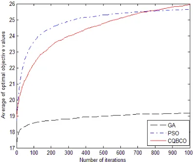
[image:8.595.205.403.507.673.2]

We can see from Fig.5, it provides the performance offered by the CQBCO approach, and we provide simulation results in terms of objective value versus number of iterations. It is obvious that the CQBCO is superior to the PSO and the GA on the average of objective value. The faster convergence rate of CQBCO is obvious.

Fig.5: Objective function performance of three algorithms with 50 elements.

We can see from Fig.6, it illustrates the performance offered by CQBCO, PSO and GA approaches, and we provide simulation results in terms of objective value verse number of iterations. It is clearly that GA has poor performance. Although it is not obvious that CQBCO is better than PSO, we can know that the average of optimal objective value of CQBCO still has a tendency to rise. So we can conclude that CQBCO outperforms PSO and GA in convergence precision. And the proposed CQBCO algorithm can overcome the disadvantages of the previous intelligence algorithms.

Fig. 6: Objective function performance of three algorithms with 200 elements.

[image:9.595.225.425.82.246.2] [image:9.595.205.402.357.520.2]

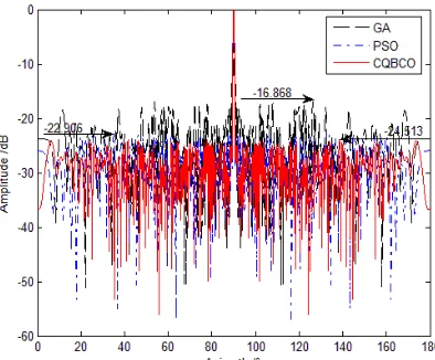
Fig.7: Amplitude performance of three algorithms with 50 elements

Fig.8 shows the amplitude

FF

( )

θ

of three algorithms with 200 elements. We provide simulation results in terms of amplitude versus azimuth. We obtained the maximum side lobe level as slow as -24.513dB when we use CQBCO, but we just obtained -22.906dB and 16.868dB maximum side lobe level when we adopt PSO and GA, respectively. Side lobe value obtained by CQBCO is 1.607dB lower than that of PSO and 7.645dB lower than that of GA. It is obvious that. CQBCO obtains a lower maximum side lobe level. It provides that CQBCO has better global convergence property and excellent maximum side lobe level.

Fig. 8: Amplitude performance of three algorithms with 200 elements.

CONCLUSION

This paper has proposed a CQBCO algorithm which is a novel algorithm for discrete optimization problems. Though testing classical benchmark functions, it can be seen that the CQBCO overcomes the disadvantage of local convergence and has much accurate convergence value, and CQBCO algorithm is superior to other classical evolutionary algorithms. It can be seen that CQBCO has a good universality, so it is easy transplanted to solve other engineering optimization problem. There is no doubt that advances in parallel computing would make CQBCO more attractive and practical for thinned array optimization.

Acknowledgments

This work was supported by the National Natural Science Foundation of China (No. 61102106), China Postdoctoral Science Foundation (No. 2013M530148), Heilongjiang Postdoctoral Fund (No. LBH-Z13054) and the Fundamental Research Funds for the Central Universities (No. HEUCF140809).

REFERENCES

[1] Kennedy, J.; Eberhart, R, Discrete binary version of the particle swarm optimization. IEEE International Conference on Computational Cybernetics and Simulation. ,1997 ,5,4104–4108,.

______________________________________________________________________________

Humans. 2012, 42(2), 511-526.

[3] Karaboga, D. ; Basturk, B., Applied Soft Computing. ,2008 ,8(1), 687-697.

[4] Liu, L.L.; Yang, S.X.; Wang D.W., IEEE Transactions on Systems, Man, and Cybernetics, Part B: Cybernetics., 2010, 40(6), 1634-1648.

[5] Wong, L.P.; Chi, Y. P.; Malcolm, Y. H. L.; Chin, S.C., Bee colony optimization algorithm with big valley landscape exploitation for job shop scheduling problems. Proceedings - Winter Simulation Conference., 2008, 2050-2058. [6] Han, K. H.; Kim, J. H., Genetic quantum algorithm and its application to combinatorial optimization problems. Proceedings of the 2000 IEEE Conference on Evolutionary Computation, Piscataway: IEEE Press., 2000, 2, 1354–1360.

[7] Yang, J.-A.; Li B.; Zhuang, Z., J. Electron. 2003, 20(1), 62–68.

[8] Gao, H.Y.; Liu, Y.Q.; Diao, M., International Journal of Innovative Computing and Applications. ,2011, 3(3),160-168.

[9] Lo, Y. T.; Lee, S.W., Aperiodic arrays, in Antenna Handbook, Theory, Applications, and Design. New York Van Nostrand. 1988.

[10] Willey, R. E., IEEE Antennas Propagat., 1962, 10(4), 369-377.

[11] Galejs, J., Minimization of sidelobes in space tapered linear arrays. IEEE Trans. Antennas Propagat., 1964, 12(4),835-836.

[12] Steinberg, B. D., Principles of Aperture and Array System Design. New York Wiley. 1976. [13] Lo, Y. T.; Lee, S. W., IEEE Trans. Antennas Propagat., 1966, 14(1), 22-30.

[14] Press W. H. et al., Numerical recipes. New York: Cambridge University Press. 1992

[15] Cheston T. C.; Frank J., Phased array radar antennas. in Radar Handbook. M. Skolnik, Ed. New York McGraw-Hil. 1990.

[16] Davis , L., Generic algorithms and simulated annealing. Los Altos, CA: Morgan Kaufmann. 1987. [17] Ruf, C.S., IEEE Trans. Antennas Propagat., 1993, 41(1), 85-90.

[18] Jiao, L.C.; Li, Y.Y.; Gong, M.G.; Zhang, X.Y., IEEE Transactions on Systems, Man, and Cybernetics, Part B: Cybernetics. , 2008, 38(5), 1234–1253.

[19] May, R. M., Nature., 1976, 261(5560), 459-467.

[20] Coelho, L. D. S., Bora, T. C., Lebensztajn, L. IEEE Transactions on Magnetics., 2012,48(2), 751-754.

[21] Zhao, Z.J., Peng, Z., Zheng, S.L., Shang, J.N., IEEE Transactions on Wireless Communications., 2009,8(9),4421-4425.

[22] Haupt,Randy L. IEEE antennas and propagation society., 1994,42(7), 993-99.