Source Processes
Thesis by Junle Jiang
In Partial Fulfillment of the Requirements for the Degree of
Doctor of Philosophy
California Institute of Technology Pasadena, California
2016
©2016
©2016
Acknowledgements
Pursuing a Ph.D. at Caltech has been a special journey for me which not only rewarded me with intellectual development, but also personal growth and a sense of cultural identity. I am truely grateful that Nadia and Mark have been the most significant people of my time at Caltech, as they were friends who imparted life experiences as well as mentors who guided my academic trainings. Nadia was the first person I turned to as a physics major, intrigued and yet perplexed by the complex geophysical world, and I always enjoyed critical thinking and discussions with her. Mark is the mastermind who provided me with first-hand and teamwork experiences of working on megathrust earthquakes over the years whenever they culpably generate tsunamis, and I appreciate that he always challenged me to think outside the box. I feel fortunate to have been involved with both of their groups and to have been introduced to unique perspectives on some geophysical problems. Indeed, the work I present in my thesis could not have been accomplished without their encouragement, support, and trust as well as patience over the years. I want to especially express my appreciation for their support in face of the adversities of my personal life; their words of advice and comfort at the time were just as precious as those of my family.
Computational Geophysics, and Jean-Philippe for the most inspiring series of Ge277 Active Tectonics seminar classes, which I still benefit from reviewing time after time.
I thank other professors at Seismo Lab, including Rob, Don, Victor, Joann, Jennifer, Hiroo, Mike, Egill, and Zhongwen for classes, field trip opportunities, discussions, and everything else. Outside the Seismo Lab, I am particularly grateful to Joe for introducing me to the Palau project, several Ge136 excursions to the Grand Canyon, Baja California etc., and leading the division enrichment trip to Japan, together with Paul and Atsuko.
I have heartfelt gratitude for many postdocs and senior members in the group who provided support and inspirations for me, in particular, Hiro, Sylvain, Anthony, Sarah, Francisco, and Zacharie, because I think parts of my thesis directly benefit from their guid-ance and foundational work. I want to thank all the group members over the years who offered great company and enjoyable exchanges: Ting, Ahmed, Surendra, Hasha, Vahe, Nina, Ravi, Marion, Brent, Semechah, Stephen, Bryan, Vito, Hilary, Romain, Jessica, Mar-cello, Srivatsan, Nadaya, Jeff, Han, and Chris; my officemates Laura, Thomas, Dunzhu, Xiaolin, Vish, Minyan, and Jack; those with whom I share lots of interesting conversa-tions and activities, Yiran, Dongzhou, and Yingdi; and everyone else in the Seismo Lab. I thank all the admins for their wonderful support and always pleasant interactions: Donna, Rosemary, Viola, Julia, Sarah, Evelina, Kim, Maria, Liz, Leticia, Priscilla, and Carolina.
I’m thankful for Michael and Hailiang for their guidance on computation and support in developing AlTar as a teamwork.
I thank Yihe and Zhihong for the most memorable times at Caltech.
I’m also thankful for my undergraduate university, Peking University, which has cast deep influence on me in ways that I appreciate greatly.
Abstract
Investigation of large, destructive earthquakes is challenged by their infrequent occurrence and the remote nature of geophysical observations. This thesis sheds light on the source processes of large earthquakes from two perspectives: robust and quantitative observational constraints through Bayesian inference for earthquake source models, and physical insights on the interconnections of seismic and aseismic fault behavior from elastodynamic modeling of earthquake ruptures and aseismic processes.
To constrain the shallow deformation during megathrust events, we develop semi-analytical and numerical Bayesian approaches to explore the maximum resolution of the tsunami data, with a focus on incorporating the uncertainty in the forward modeling. These methodolo-gies are then applied to invert for the coseismic seafloor displacement field in the 2011Mw 9.0 Tohoku-Oki earthquake using near-field tsunami waveforms and for the coseismic fault slip models in the 2010Mw 8.8 Maule earthquake with complementary tsunami and geode-tic observations. From posterior estimates of model parameters and their uncertainties, we are able to quantitatively constrain the near-trench profiles of seafloor displacement and fault slip. Similar characteristic patterns emerge during both events, featuring the peak of uplift near the edge of the accretionary wedge with a decay toward the trench axis, with implications for fault failure and tsunamigenic mechanisms of megathrust earthquakes.
Contents
Acknowledgements iv
Abstract vii
1 Introduction 11
2 Bayesian Inference of Coseismic Seafloor Deformation During the 2011 Tohoku-Oki Earthquake with Near-field Tsunami Waveforms 15
Abstract 16
2.1 Introduction . . . 18
2.2 Tsunami observations and modeling . . . 21
2.2.1 Observations of the 2011 Tohoku-Oki earthquake induced tsunami . 21 2.2.2 Model parameterization of seafloor deformation and tsunami excitation 23 2.2.3 Forward modeling of the tsunami propagation . . . 26
2.3 Bayesian inference of seafloor deformation model . . . 29
2.3.1 Bayesian formulation of the inverse problem . . . 29
2.3.2 Semi-analytical approach for the quasi-static problem . . . 30
2.3.3 Sampling approach for the kinematic problem . . . 31
2.3.5 Posterior uncertainty and resolution analysis . . . 34
2.4 Synthetic scenarios . . . 36
2.5 Applications to the 2011 Tohoku-Oki earthquake . . . 42
2.5.1 Quasi-static seafloor deformation models . . . 42
2.5.2 Kinematic seafloor deformation models . . . 43
2.6 Discussion . . . 50
2.6.1 The resolution of tsunami data . . . 50
2.6.2 Assumptions and advantages of our methodology . . . 51
2.6.3 Seafloor deformation and fault slip near the trench . . . 52
2.7 Conclusion . . . 60
Appendices 62 2.A Frequency dispersion in tsunami propagation . . . 62
2.B Different formulations of Cp for tsunami waveforms . . . 64
3 A Bayesian Perspective on the Complementarity of Tsunami and Geode-tic Observations for the 2010 Mw 8.8 Maule, Chile Earthquake 71 Abstract 72 3.1 Introduction . . . 74
3.2 Data and methods . . . 75
3.2.1 Fault geometry and model parameterization . . . 75
3.2.2 Geodetic observations and modeling . . . 76
3.2.3 Tsunami observations and modeling . . . 76
3.2.4 Semi-analytical Bayesian approach to fault slip models . . . 79
3.3 Results and discussions . . . 83 3.3.1 Fault slip models from tsunami, geodetic, and joint inversions . . . . 83 3.3.2 Effects of dispersion, elastic structure, and error models . . . 89 3.3.3 Updip and downdip resolution of fault slip . . . 97 3.4 Conclusion . . . 99
4 Deeper Penetration of Large Earthquake Ruptures on Seismically
Quies-cent Faults 103
Abstract 104
4.1 Main Text . . . 105
Appendices 116
4.A Materials and Methods . . . 116 4.A.1 Earthquake catalogues and coseismic slip models . . . 116 4.A.2 Microseismicity vs. depth extent of earthquakes from slip models . . 117 4.A.3 Paleoseismic Records for the San Andreas and San Jacinto Faults . . 123 4.A.4 Numerical methods and model setup . . . 132 4.B Supplementary Text . . . 137 4.B.1 Physical mechanisms favoring or discouraging deeper coseismic slip . 137 4.B.2 Long-term fault behavior in numerical simulations . . . 138 4.B.3 Estimating the migration of stress concentration front . . . 140
5 Connecting Seismicity, Fault Locking and Large Earthquake Rupture at
Depth 154
5.1 Introduction . . . 157
5.2 Model setup . . . 159
5.3 Seismic and aseismic behavior in long-term fault models . . . 160
5.3.1 Large earthquake rupture and seismicity . . . 160
5.3.2 Fault coupling and geodetically-estimated fault locking depth . . . . 164
5.3.3 Spatial relations and temporal evolutions of different depths . . . 168
5.4 Inferring the geodetic locking depths on major faults . . . 170
5.5 Seismicity and fault heterogeneity at the transitional depth . . . 175
5.6 Conclusion . . . 179
List of Figures
2.1 Source region and tsunami records for the 2011 Tohoku-Oki earthquake . . . 22 2.2 Parameterization of the seafloor deformation and forward modeling of tsunami
excitation and propagation. . . 25 2.3 Design of the variance-covariance matrix for the model prediction error Cp . 35 2.4 Inversions of a synthetic scenario with maximum seafloor uplift away from the
trench . . . 40 2.5 Inversions of a synthetic scenario with maximum seafloor uplift at the trench 41 2.6 Spatial averaging of posterior solutions and model uncertainties . . . 42 2.7 Spatial averaging and uncertainty analysis of the posterior solutions. . . 44 2.8 Posterior mean models for the quasi-static problem with different Cp . . . . 45 2.9 Posterior data fit and prediction of later waveforms for the quasi-static solutions. 46 2.10 The uncertainty, averaging scale, and original posterior mean models for the
kinematic problem. . . 48 2.11 The uncertainty, averaging scale, and 1R-averaged posterior mean models for
the kinematic problem. . . 49 2.12 Posterior data fit and prediction of later waveforms for the kinematic solutions. 50 2.13 Seafloor deformation near the trench in the kinematic model and comparisons
2.14 Probabilistic characterization of the near-trench seafloor tilt . . . 56 2.15 Seafloor deformation near the trench in the quasi-static model . . . 57 2.16 2D subduction zone models with different elastic structure and bathymetry . 59 2.17 Seafloor uplift and subsurface fault slip in 2D elastic models . . . 60 2.18 The original and filtered tsunami waveforms . . . 67 2.19 Frequency dispersion relations for tsunami propagation . . . 68 2.20 The effect of water layer attenuation and wave dispersion on tsunami GF . . 68 2.21 Different formulations of Cp for tsunami forward modeling . . . 69 2.22 Great-circle path and ray path approximations in tsunami propagation . . . 70
3.1 Fault geometry and station distribution for the 2010 Mw 8.8 Maule earthquake 77 3.2 The reference velocity model and perturbed models . . . 83 3.3 Cχ for the geodetic (GPS & InSAR) and tsunami modeling . . . 84
3.4 Coseismic fault slip models from tsunami, geodetic, and joint inversions with
Cχ . . . 87
3.5 Predicted surface displacement from tsunami, geodetic, and joint models with
Cχ . . . 88
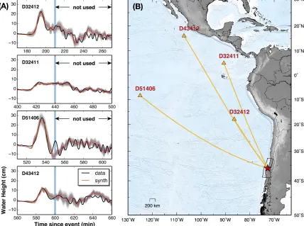
3.6 Observed and predicted InSAR measurements using the favored joint models 90 3.7 Observed and predicted GPS displacements using the favored joint models . 92 3.8 Observed and predicted DART waveforms using the favored joint models . . 93 3.9 The effect of elastic structure and error models on geodetic inversions . . . . 94 3.10 The effect of dispersion and error models on tsunami inversions . . . 95 3.11 Coseismic fault slip models from tsunami, geodetic, and joint inversions with
3.12 The trench-normal profile of surface displacements predicted from the favored
joint models . . . 100
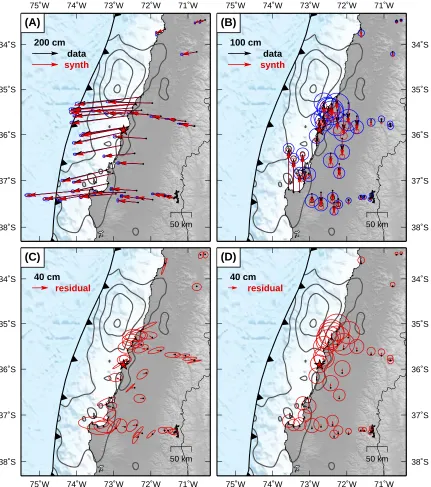
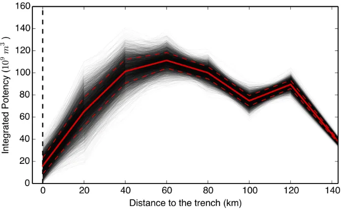
3.13 Along-strike integrated seismic potency . . . 101
3.14 Comparisons between co- and post-seismic fault slip models and aftershocks . 102 4.1 Schematic illustration of our fault model and the locked-creeping transition . 106 4.2 Observations of large earthquakes and microseismicity patterns on major strike-slip faults . . . 107
4.3 Microseismicity and the potential for deeper ruptures on the San Andreas Fault (SAF) and the San Jacinto Fault (SJF) in Southern California . . . 108
4.4 The relation between the depth extent of large earthquakes and microseismicity in simulated earthquake sequences . . . 112
4.5 2004 Mw 6.0 Parkfield and 1984 Mw 6.3 Morgan Hill earthquakes . . . 124
4.6 1979 Mw 6.4 Imperial Valley and 1987Mw 6.7 Superstition Hills earthquakes 125 4.7 1989 Mw 7.1 Loma Prieta earthquake . . . 125
4.8 1999 Mw 7.6 Izmit earthquake . . . 126
4.9 2002 Mw 7.9 Denali earthquake . . . 127
4.10 2001 Mw 7.9 Kokoxili earthquake . . . 128
4.11 1906 Mw 7.9 San Francisco earthquake . . . 129
4.12 Uncertainty of earthquake locations . . . 130
4.13 Depth dependence of rate-and-state frictional properties and normal stress . 135 4.14 Illustration of the locations of the along-depth profiles and observation points 139 4.15 Accumulated fault slip along depth over several large earthquakes . . . 141
4.18 Time evolution of the along-depth shear stress and slip rate profiles in model
M1 . . . 144
4.19 Time evolution of the along-depth shear stress and slip rate profiles in model M2 . . . 145
4.20 Post- and inter-seismic migration of the SCF after a deeper-penetrating event. 147 4.21 Post- and inter-seismic response of faults with different frictional properties at depth . . . 151
4.22 Post- and inter-seismic fault slip and the migration of SCF . . . 152
4.23 Dependence of migration distanceDprop of the SCF on ∆τeq andaσ . . . 153
5.1 Seismicity and geodetic locking depths on the San Andreas and San Jacinto faults . . . 158
5.2 Conventional elastic dislocation model for earthquake cycles . . . 159
5.3 Fault models with different frictional properties at the seismic-aseismic transition161 5.4 Distribution of large earthquake slip and seismicity in the long-term fault models162 5.5 The depth distributions of stress, stressing, fault slip tand seismicity . . . 165
5.6 Time evolution of fault coupling in the interseismic periods . . . 166
5.7 Time-dependent fault slip rates at depth and surface velocity . . . 168
5.8 Inversion of the locking depth Dgeod and fault slip rateVcr . . . 169
5.9 Time dependence ofDlock,Dgeod, and D0.5C in the interseismic period . . . . 171
5.10 The effect of layered elastic structure on the inference of Dgeod and Vcr . . . 173
5.11 Illustration of slip partition and Dgeod,Dseis Dlock, and Drupt in a seismic cycle 175 5.12 Conceptual and physical models for faults with other heterogeneity . . . 177
5.13 Complex fault behavior and variation of fault coupling in model M5 . . . 178
List of Tables
2.1 Summary on the characteristics of different Cp . . . 67
4.1 Coseismic slip models and catalogues for events that satisfy our selection criteria.118 4.2 Calendar years for historical and prehistorical earthquakes (after A.D. 1000)
Chapter 1
Introduction
Since the elastic rebound theory was first put forth by Harry Fielding Reid in 1910, shortly after the devastating 1906 San Francisco earthquake in Northern California, the phenom-ena of earthquakes in the shallow crust have been well recognized as a major behavior of tectonic faults to release strain energy, which is stored during long-term stasis, through rapid displacements across the fault. The nature of recurrence and virtual unpredictability of earthquakes makes them a formidable natural hazard.
Modern geophysical observations, including seismological instruments and geodetic tech-niques that measure crustal deformation over a wide range of spatial and temporal scales, have been enriching our experiences and understandings of earthquakes and fault behavior. Among all, large earthquakes are rare occurrences and often are more challenging to observe due to their remoteness. In major subduction zones, fault slip during megathrust events occurs offshore, but the induced tsunami still bears a significant impact on the coast. Large continental earthquakes usually initiate deep in the seismogenic zone of faults, under the extreme conditions that are still beyond the reach of the most advanced drilling techniques and borehole observations.
Japan. Some of them came with surprising features, with the 2011 Mw 9.0 Tohoku-Oki earthquake as a notable example, which occurred in unanticipated locations with much underestimated impact from the induced tsunami (Simons et al., 2011). The event serves as a constant reminder for us that predicting the behavior of earthquakes is a challenging task. How these rare earthquakes behave provides us with valuable and vital information for solving their mystery, thus motivating quests into understanding the detailed coseismic physical processes, and also leading to studies of other closely related phenomenon – af-tershocks, postseismic afterslip, viscoelastic and poroelastic bulk relaxations, etc. (Segall, 2010) – which have now been routinely carried out after major earthquakes.
For another type of major fault systems – continental strike-slip faults – we still have limited experiences of large earthquakes in heavily-populated modern urban regions. As one of the most prominent faults of this type in a well-instrumented and well-studied region, the San Andreas Fault in California has not had an event of Mw > 7 since the 1906 temblor in Northern California, and not since the 1857 Mw 7.9 Fort Tejon earthquake in Southern California, with an even more overdue Coachella segment at the southernmost end, which sits in peace since ∼ 1690 (WGCEP, 1995). Paleoseismic studies continue to reveal more information about these past events (e.g.,Sieh, 1978a;Zielke et al., 2010), which complements our current observations which are limited to only several decades of seismic monitoring and over a decade of quality geodetic measurements for the late interseismic period of faults.
so-called rate-and-state friction laws, in which earthquakes occur as slip instability that develops under loading (Dieterich, 2007). Such a framework gains acceptance and valida-tion through many successful applicavalida-tions for understanding the recurrence of earthquakes, depth variation of fault slip, etc. (Scholz, 2002). Among many important implications, it is suggested that aseismic processes can influence the initiation, i.e. nucleation, of earthquakes. Recent experiments under high velocity conditions further reveal a variety of mechanisms through which enhanced dynamic weakening could occur (Tullis, 2015), alluding to the fur-ther complexity in the earthquake process that their nucleation and rupture are potentially governed by different mechanisms. On tectonic faults, they might be interconnected through aseismic processes. Understanding how these laboratory findings connect with large-scale earthquake phenomena and how their combinations with theories can guide us in the real world requires comparing model predictions with different lines of observations.
This thesis consists of two main parts in which we develop new observational and physical approaches to understand the earthquake source processes. Our studies focus on two typical tectonic settings where large earthquakes occur: the megathrust faults in subduction zones (Chapter 1 and 2), and continental mature strike-slip faults (Chapter 3 and 4).
depend on robust and well-characterized source models.
In Chapter 2, we explore the complexity in the finite-fault slip inversions for the 2010 Mw 8.8 Maule, Chile earthquake with joint use of geodetic and tsunami observations. Pre-viously published models based on different types of datasets feature large discrepancies in the locations of the peak slip and slip near the trench, even though, in this case, the trench-to-coast distance is evidently shorter than in Japan. Using the Bayesian formulation, we aim to understand the complementarity and respective roles of tsunami and geodetic data in inferring the final joint models and the significance of model prediction uncertainty associated with each of them, and to eventually better understand the shallow slip process during this event and compare it with the Tohoku-Oki earthquake.
In Chapter 3, we focus on the long-standing enigma of seismic quiescence on several fault segments of the San Andreas Fault in California, and on other mature faults. We resort to dynamic modeling of the interactions between large earthquake rupture, microseismicity, and aseismic slip in fault models with laboratory-derived friction laws, and combine physical insights with observational clues to understand the phenomena of deeper penetration of large earthquakes below the seismogenic zones on these mature faults, with implications for fault rheology and earthquake scaling.
Chapter 2
Abstract
To improve our understanding of the source process during the 2011 Mw 9.0 Tohoku-Oki earthquake, we develop an approach to invert for seafloor deformation using only tsunami waveforms recorded by a variety of near-field instruments. Our Bayesian formulation allows us to explore the maximum resolution of the tsunami data, and to investigate still unresolved questions such as the extent of near-trench seafloor displacement and inferred shallow fault slip. In this analysis, we place special focus on the error structure used in the inverse problem. By focusing purely on seafloor displacements and not on subsurface fault slip, we avoid the need to address common sources of uncertainties, such as fault geometry and spatial variations in elastic structure encountered in conventional fault slip inversions. For the quasi-static problem, we adopt a semi-analytical Bayesian approach to derive closed-form expressions for the posterior solutions of seafloor displacement with minimal a priori
2.1
Introduction
The 2011 Mw 9.0 Tohoku-Oki earthquake is one of the most destructive and best docu-mented megathrust events. Its location, extent of rupture, and induced tsunamis provide us a unique opportunity to study the mechanisms of a great earthquake.
static and/or kinematic data (Ammon et al., 2011; Hayes, 2011; Koketsu et al., 2011; Si-mons et al., 2011;Yokota et al., 2011;Romano et al., 2012, 2014;Wei et al., 2012;Yue and Lay, 2013; Bletery et al., 2014; Minson et al., 2014).
The joint inversions produce several consistent scale features, including large-amplitude fault slip updip of the hypocenter that reaches the trench. However, these models still disagree in ways that have important implications for fault mechanics and source physics. For example, they differ in the inferred location and thus the depth of peak fault slip and the profile of near-trench seafloor deformation. Here, we are particularly con-cerned with the range of source models that can be resolved by the tsunami data within the uncertainty of seafloor geodetic measurements. These questions remain unresolved, with im-portant implications for hazard analyses as well as on follow-up studies such as calculations of stress interactions, postseismic afterslip, and bulk relaxation near the trench.
adopted in the inversion critically influences our inference. Here, we explicitly consider the model prediction error due to uncertainties in the physics of tsunami propagation, in addition to the relatively insignificant observational error due to imprecise measurements. We adopt a Bayesian formulation of the inverse problem to derive the posterior solutions, from which uncertainty and resolution are readily assessed. Since this approach does not explicitly involve fault slip, the impact of other processes, e.g., submarine landslides, are in principle included. Our efforts to decouple the tsunami excitation problem from the finite-fault slip inversions and to explore the error structure and resolution of tsunami waveforms are the first step toward a more complete and consistent integration with other types of datasets and other sources of uncertainty (e.g., elastic properties).
assump-tions, implications for coseismic seafloor deformation and fault slip near the trench, and the value of a probabilistic view for source models.
2.2
Tsunami observations and modeling
2.2.1 Observations of the 2011 Tohoku-Oki earthquake induced tsunami
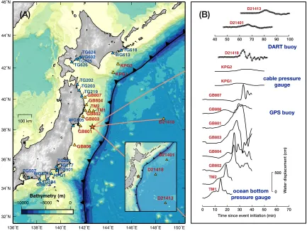
The tsunami generated by the 2011 Tohoku-Oki earthquake was observed by a variety of modern seafloor and ocean surface instruments, making the event unique for the diverse, comprehensive, and high-quality available tsunami records. Near the source region, ocean bottom pressure gauges, e.g., TM1 and TM2 in Maeda et al.(2011), recorded the earliest arrivals and the largest amplitude of the traveling tsunami waves. Closer to the coast, these waves were also recorded by cable pressure gauges (e.g, www.jamstec.go.jp/scdc/top_
e.html) on the seafloor and GPS gauges (NOWPHAS,nowphas.mlit.go.jp/index_eng. html), which are tethered to the seafloor and record the water height. Coastal water gauges and tide gauges record these incoming tsunami waves and interactions of the tsunami with local features. In the open ocean, the long-wave tsunamis are recorded by the DART® (Deep-ocean Assessment and Reporting of Tsunamis) tsunameters in the Pacific. The distribution of these near-field stations is shown in Fig. 2.1A.
100 km
136˚E 138˚E 140˚E 142˚E 144˚E 146˚E 148˚E 150˚E
32˚N 34˚N 36˚N 38˚N 40˚N 42˚N 44˚N 46˚N TM1 TM2 GB802 GB804 GB803 GB801 GB806 KPG1 KPG2 D21418 GB807 HPG1 GB812 TG202 TG203 WG205 TG217 TG219 TG221 WG501 TG504 TG507 WG602 WG613 TG618 TG624 TG625 TG626 TG901
−10000 −5000 0
Bathymetry (m) D21418 D21401 D21413 GPS buoy ocean bottom pressure gauge DART buoy cable pressure gauge
(A)
(B)
5000 Water displacement (cm)
Time since event initiation (min) 0 10 20 30 40 50 60 70
[image:30.612.107.540.175.500.2]40 50 60 70 80 90 100
have higher sampling rates at 5 seconds. DART records, lowpass-filtered at 2 minutes, and other waveforms at 60 seconds, are shown in Fig. 2.1B (the original and filtered waveforms in Fig 2.18). All waveforms are offset to start at zero displacement at the initiation time of the earthquake. We use the 30-40 minutes of each waveform that include only the first arrivals, thereby avoiding complex wave interactions with coastal reflections in later wave-forms. These recordings form a unique dataset in the near field of the source with good azimuthal coverage.
2.2.2 Model parameterization of seafloor deformation and tsunami
exci-tation
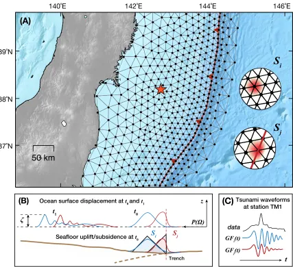
We parameterize our model of the seafloor deformation field (positive values for effective uplift and negative for effective subsidence) without explicit consideration of the underlying causal physical process, as illustrated in Fig. 2.2A. We consider an area of the seafloor which spans from the coastline to a limited distance seaward of the trench. We then discretize each side of the trench into a triangulated surface with an unstructured grid, using split nodes on the trench where the two meshes meet. From the triangulated meshes we construct overlapping piece-wise linear (tent) functions centered on each node, including full-tents for the interior nodes (Si) and half-tents for boundary nodes, including those on the trench (Sj). Following Geist and Dmowska (1999), we then apply a spatial filter 1/tanh (kh) to the source to reduce short-wavelength features that would normally be attenuated by the water layer (Kajiura, 1981) (the effect of such attenuation on the resultant waveform GFs is shown in Fig. 2.20), and then renormalize all the smoothed sources to unit peak uplift for use in the forward modeling.
im-posed on the nodes (Simons et al., 2011). Offshore nodes on the boundary of the mesh are set to zero and are thus assumed to be beyond the region of significant seafloor deformation. We do not impose values on nodes at the trench, so that nonzero uplift at the trench is allowed. Such a parameterization has several advantages relative to a conventional quadri-lateral based parameterization: (1) The triangulated surface honors the curved shape of the trench line; (2) When compared to a piece-wise constant parameterization, the smoothed tent function is a physically realistic representation of the source of tsunami excitation with the advantage of being numerically stable in the wave propagation model; (3) The smoothed half-tent function still allows relatively sharp deformation features at the trench.
ζ
z
P(Ω)
Tsunami waveforms at station TM1
t0
t1
Sj
Si
Ocean surface displacement at t0 and t1
t
GFi(t)
GFj(t) data
Trench
Seafloor uplift/subsidence at t0
50 km
140˚E 142˚E 144˚E 146˚E
37˚N 38˚N 39˚N
S
iS
j(A)
[image:33.612.112.539.129.519.2](B)
(C)
spite of the short duration and compact size of the event, which is usually used to justify the quasi-static treatment. Here we consider both the quasi-static and kinematic formulations.
2.2.3 Forward modeling of the tsunami propagation
Numerical methods based on linear or nonlinear shallow water wave equations (e.g., COM-COT, Liu et al., 1995) are generally effective and computationally efficient in simulating tsunami waveforms in the open ocean, as are recorded at DART stations. However, it is more challenging to simulate tsunami propagation in the near-source and coastal regions with shallower water depth. Nonlinear effects become increasingly important, and we can no longer neglect finite wave amplitude, ocean stratification, Coriolis forces, and bottom friction. The assumption of long waves in the shallow water equation can break down, requiring a more appropriate Boussinesq type formulation (Peregrine, 1967) or even fully hydrodynamic simulations. Frequency dispersion is also an important characteristic of the tsunami propagation process. Even in the long-wave (long period) limit in the open ocean, far-field tsunami dispersion has been recognized to play an important role in delayed travel times and responsible for the initial reversed polarity in many waveforms observed during recent large earthquakes, including the 2011 Tohoku-Oki event (Tsai et al., 2013; Watada, 2013; Watada et al., 2014). These dispersion effects can be included numerically (Allgeyer and Cummins, 2014) or empirically (Yue et al., 2014). Dispersion also occurs in the short wave (short period) limit and can produce features not captured in simplified waveform modeling.
500-meter bathymetry (http://www.jodc.go.jp/data_set/jodc/jegg_intro.html) for near-field stations and ETOPO1 bathymetry (Amante and Eakins, 2009) for DART. In both cases, we use a grid spacing of 500 m. We also consider the uncertainty in the modeling of tsunami propagation associated with different assumptions with respect to dispersion. In Appendix A, we summarize the variability of frequency dispersion relations for different tsunami problems, as they will be useful when we consider modeling uncertainties (Sec-tion 2.3.4).
For the quasi-static problem, we assume that seafloor deformation and tsunami excita-tion occur instantaneously over the entire source region, with no time delay beween sources. For the kinematic problem, we consider time-dependent seafloor displacement by assuming a spatially variable local propagation velocity governed by an Eikonal equation:
|∇t0(x, y)|= 1/vr(x, y), (2.1)
where t0 is the initiation time of seafloor deformation at location (x, y) and equals 0 at the epicenter location, and vr is the velocity of the deformation front corresponding to the apparent rupture velocity of the earthquake, which we call the displacement propagation velocity for simplicity. We assume a triangular function with a half-width of 30 sec for the displacement rate at each source, and divide the entire event duration into 8 time windows of 30 sec each. For a given distribution of non-uniformvr, we solve fort0 in Eq. 2.1 on the triangular mesh using the Fast Iterative Method on GPU (Graphics Processing Unit) (Fu et al., 2011), and the initiation time of each source of displacement is assigned to be the beginning of the corresponding time window for t0.
station. Synthetic waveforms are generated as a linear combinations of these Green’s func-tions without or with a time shift for quasi-static and kinematic problems, respectively (Fig. 2.2B-C). Both observed and simulated waveforms are offset to zero at the origin time. The linearity of the forward problem is commonly assumed in source inversions of tsunami waveforms (Satake and Tanioka, 1999), and is generally valid for recordings some distance away from the coast. Thus in matrix form we have:
d= [H1(ts1), ..., H1(te1), ..., HN(tsN), ..., HN(teN)]T
m=U1, U2, ..., UM
G=
G1,1(ts1+T1) · · · G1,2(ts1+T2) · · · G1,M(te1+TM) ..
. . .. ... ...
G1,1(te1+T1) · · · G1,2(t1e+T2) · · · G1,M(te1+TM) ..
. ... . .. ...
GN,1(teN +T1) · · · GN,2(teN+T2) · · · GN,M(teN +TM)
,
where the data vector d consists of concatenated records from N stations with Hi(t) for respective time windows [ts
i, tei] (i = 1, ..., N) (superscripts s and e indicate the start and the end of the time series, respectively), with time shift Tj (j = 1, .., M) corresponding to different sources, the vectormconsists of M seafloor uplift/subsidence sourcesUk (k= 1, ..., M), andGis the Green’s function matrix, containing Green’s functionGi,j(t) between station i and source j. The quasi-static problem with Ti = 0 is linear with respect to the total model parameter vector θ(θ=m). Even though the kinematic problem is nonlinear
with respect to the model θ = [m,vr] which includes displacement propagation velocity
of time shifts, which has computational advantages. For both quasi-static and kinematic problems, the predicted data isdpred=G(θ) =G·m.
2.3
Bayesian inference of seafloor deformation model
2.3.1 Bayesian formulation of the inverse problem
We adopt the Bayesian formulation of the inverse problem to explore the parameter space of the model constrained by the data and our prior knowledge, as expressed in Bayes theorem (Bayes and Price, 1763):
P(θ|d)∝P(d|θ)P(θ), (2.2)
where the posterior probability distribution, P(θ|d), is proportional to the product of the
data likelihood P(d|θ), a measure of how well the model θ predicts the observed data d,
and the prior probability distribution P(θ) that reflects a priori information on model
parameters.
Assuming normal (Gaussian) distributions for all uncertainties in the problem, which is justifiable by the principle of maximum entropy (e.g.,Jaynes, 2003; Beck, 2010), the data likelihood is expressed as:
P(d|θ)∝exp−(G(θ)−d)TC−χ1(G(θ)−d), (2.3)
is usually ignored or underestimated. For large-scale problems, the variances of Cp can overwhelm those of Cd and may contain significant spatial and/or temporal correlations.
2.3.2 Semi-analytical approach for the quasi-static problem
For the seafloor deformation problem, uplift (positive values) and subsidence (negative values) are both possible and equally likely. Therefore it is reasonable to assume a normal prior:
P(m)∝exp
−(m−m0)TCm−1(m−m0)
, (2.4)
wherem0is a prior mean model, chosen as0, suggesting a preference toward no deformation in the absence of data, andCmis the prior model covariance matrix, and could be a diagonal
matrix with uniform variance if we assume constant and uncorrelated uncertainty for and no correlation between all model parameters. Increasing the variance in Cm results in a
less informative prior.
Combining Eq. 2.4 with Eq. 2.3, the posterior distribution is given as:
P(m|d)∝exp
−(G(m)−d)TCχ
−1(G(m)−d)−(m−m
0)TC−m1(m−m0)
(2.5)
∝exp
−(m−m˜)TC˜m−1(m−m˜)
, (2.6)
where m˜ is the posterior mean model, equivalent to the maximum a posteriori (MAP) model in this case, and C˜m is the posterior model covariance matrix, with the following
expressions (Tarantola, 2005, Chapter 3):
˜
m= (GTC−χ1G+Cm−1)−1(GTC−χ1d+C −1
mm0) (2.7)
˜
Cm= (GTC−χ1G+Cm
Compared with the traditional optimization approach, the expression for the Bayesian posterior mean model (Eq. 2.8) is equivalent to the maximum likelihood estimate (MLE) in the (weighted) damped least-square problem, with a regularization term that reduces the model size (Aster et al., 2013, Chapter 4). In the least-square case, the conventional least-square optimization approach is a special case of the Bayesian approach.
2.3.3 Sampling approach for the kinematic problem
In the case of a non-linear forward model, we do not have an analytic solution and must rely on sampling approaches to estimate solutions to the inverse problem. Sampling of the Bayesian posterior in high dimensional space is computationally demanding. Here we adopt the CATMIP (Cascading Adaptive Tempered Metropolis In Parallel) algorithm (Minson et al., 2013), based on the Transitional Markov chain Monte Carlo, which makes it possible to sample hundreds of model parameters efficiently with reasonable computational resources. We use the AlTar software suite, which is a reimplementation of CATMIP for hybrid CPU-GPU platforms. The CATMIP algorithm and AlTar software have previously been successfully applied to problems of finite-fault earthquake slip (Simons et al., 2011;
Minson et al., 2013, 2014;Duputel et al., 2015), interseismic fault creep (Jolivet et al., 2015), and problems in oceanography (Miller et al., 2015).
total of approximately 107 models to explore in the parameter space.
2.3.4 Design of the model prediction error Cp
The error structure of the problem, characterized by the total variance-covariance matrix
Cχ, plays a significant role in determining the data likelihood function and the eventual
posterior distribution (Eq. 2.3). Cdis usually well known, and is independent of the source. In contrast, Cp is generally expected to scale with the source, and is more difficult to characterize and quantify (Duputel et al., 2014). For a large event, such as the Tohoku-Oki earthquake, the nominal observational errors for these tsunami recordings are on the order of several cm, while the model prediction error could be much larger, given that the maximum waveform amplitudes reach several meters. Ignoring, under-estimating, or drastically mischaracterizingCpcan lead to over-fitting of data as well as biases in solutions and uncertainty estimates (see Section 2.4). The appropriate formulation of Cp is essential and thus designing Cp is a major component of this study.
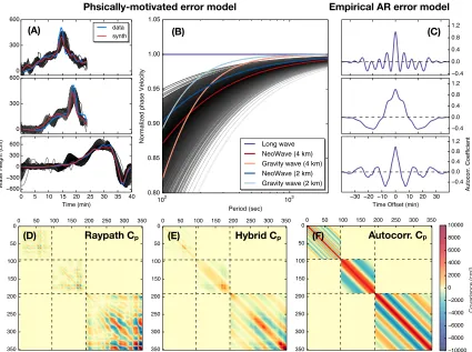
Without regard to the specific forward models, there are several empirical ways to ac-count for modeling errors. An over-simplified approach adopts a diagonalCp with inflated variances but then ignores important temporal correlations of the tsunami waveforms con-tained in the off-diagonal terms. A more reasonable approach assumes an auto-regressive error model for the time series of tsunami waveforms, resulting in a banded-Toeplitz Cp with a characteristic correlation length based on the auto-correlation function of waveform residuals.
relations. In Fig. 2.3, we illustrate our procedure to devise a physics-based formulation of
the error models. We include a more comprehensive discussion about various formulations of Cp in Appendix B, with comparisons shown in Table 2.1 and Fig. 2.21.
2.3.5 Posterior uncertainty and resolution analysis
The Bayesian formulation explicitly provides the uncertainty and correlation of model pa-rameters in the posterior solutions. Intuitively, we expect that uncertainties increase as we reduce the assumed patch size in the model, as would anti-correlation between nearby patches. However, we can always explore the PDF of local averages of the posterior solutions to learn the resolution scales inherent to the problem.
For the quasi-static problem, the posterior mean model m˜ and the posterior model covariance matrix C˜m are obtained in closed-form expressions, and hence the posterior
solutions with ad hoc spatial averaging can be derived semi-analytically:
˜
m1R=S1Rm˜ (2.9)
˜
C1Rm =S1RC˜m(S1R)T, (2.10)
whereS1R is a spatial averaging operator that averages each node value with all its nearest “one-ring” (1R) neighboring nodes (defined as nodes connected through only one edge line), andm˜1RandC˜1R
m are the corresponding posterior mean and covariance matrix in solutions
(C)
Covariance (cm
2)
Phsically-motivated error model Empirical AR error model
Autocorr. Cp
Raypath Cp Hybrid Cp
(D)
(A) (B)
[image:43.612.111.536.165.482.2](E) (F)
further reducing model uncertainties at the expense of reduced spatial resolution. For the kinematic problem, we have a posterior ensemble of models, from which m˜ and C˜m can be
computed, and we can either use Eq. 2.9 and 2.10, or apply spatial averaging directly on the sample set of the model ensemble.
For the Gaussian posterior in our case, the uncertainty Ei of model parameter mi is obtained from the posterior variance-covariance matrix:
Ei =
q
(C˜m)i,i. (2.11)
The spatial averaging operator (e.g., S1R) imposes a minimum length scale Dsi, which we choose as an effective circular diameter for the area of spatial averaging:
Dsi = 2
s
(X j
Aj+Ai)/π, (2.12)
where the summation is over all the neighboring nodes of parameter mi (based on 1R, 2R or other spatial averaging criteria), andAj is the effective tent area for node j. The impact of averaging m˜ and C˜m wil be illustrated first using synthetic scenarios.
2.4
Synthetic scenarios
features to be well-resolved while large-scale features may not be when the latter solution is in the null space. Therefore, we use some potentially realistic scenarios in these synthetic tests, and simply aim to obtain a qualitative assessment of the data resolution and an intuitive understanding of how different assumptions of source kinematics and error models might influence the results.
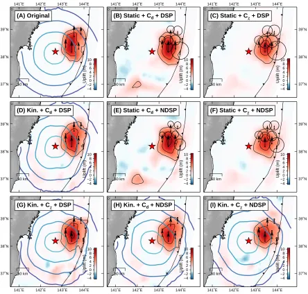
We consider two synthetic source models both of which are kinematic. The two scenar-ios differ in the proximity of maximum uplift to the trench (Figs. 2.4A and 2.5A). In both scenarios, we generate synthetic data with dispersive GF, and consider alternatively quasi-static and kinematic inversions with different combinations of Cd and Cp, and dispersive (DSP) and non-dispersive (NDSP) GF, i.e., a total of eight synthetics. Using non-dispersive GF for a dispersive propagation scenario is motivated by the fact that in real cases, we an-ticipate inaccuracy and limitations of our GF, which makes it necessary to use Cχ instead
hypocenter location of the Tohoku-oki earthquake (Chu et al., 2011).
In Fig. 2.6, we first demonstrate the effect of spatial averaging on the posterior solutions, including the mean value and uncertainty, using the posterior of a synthetic scenario in which a compact source of uplift occurs near the trench. The posterior mean model becomes smoother with the increase in the range of spatial averaging, accompanied by the reduction of error ellipses associated with the parameters highlighted. In principle, we can apply spatially nonuniform adaptive averaging based on desired resolution or criterion on the absolute or relative uncertainty, in order to eliminate null solutions where the model is less constrained and produce representative models useful for geophysical interpretations. In most of our models, we find that 1R spatial averaging is sufficient to reduce uncertainty to acceptable values and produce appropriate resolution for the source region of our interest, so we adopt the uniform 1R spatial averaging in this study. In Figs. 2.4 and 2.5, all posterior solutions are shown after 1R averaging.
From the results of synthetic tests, we find that inversions of quasi-static models with only Cd tend to bias the solutions toward more localized and larger uplift with peak value offset in space from the input model (Figs. 2.4B,E and 2.5B,E). Spurious features of subsi-dence to the south are also observed in these models, and are particularly bad in Fig. 2.5B,E, because source kinematics and the dispersive nature of tsunami both introduce waveform complexity, and ignoring finite displacement propagation velocity would force these addi-tional features into the model in order to fit the waveform, as is also reported by Hossen et al. (2015). Such a bias is amplified for the case of a more dispersive tsunami wave ex-cited at the trench (see Fig. 2.20). However, we observe that with the incorporation of more realistic Cχ (Figs. 2.4C,F and 2.5C,F), the bias due to the quasi-static assumption is
is more compatible with the true model within uncertainty. In the quasi-static problem, we notice that by using NDSP GFs (Fig. 2.4E,F and 2.5E,F), not only are spurious features worse, but uncertainties are also underestimated more than their counterparts with DSP GF (Fig. 2.4B,C and 2.5B,C), suggesting that an inaccurate GF without an appropriateCp can lead to a biased mean solution and underestimated uncertainties.
50 km
141˚E 142˚E 143˚E 144˚E
37˚N 38˚N 39˚N (A) Original −4 −2 0 2 4 6 8 10 Uplift (m) 50 km
141˚E 142˚E 143˚E 144˚E
(B) Static + Cd + DSP
−4 −2 0 2 4 6 8 10 Uplift (m) 50 km
141˚E 142˚E 143˚E 144˚E
37˚N 38˚N 39˚N
(C) Static + Cχ + DSP
−4 −2 0 2 4 6 8 10 Uplift (m) 50 km 37˚N 38˚N 39˚N
(D) Kin. + Cd + DSP
−4 −2 0 2 4 6 8 10 Uplift (m) 50 km
(E) Static + Cd + NDSP
−4 −2 0 2 4 6 8 10 Uplift (m)
50 km 37˚N
38˚N 39˚N
(F) Static + Cχ + NDSP
−4 −2 0 2 4 6 8 10 Uplift (m) 50 km
141˚E 142˚E 143˚E 144˚E 37˚N
38˚N 39˚N
(G) Kin. + Cχ + DSP
−4 −2 0 2 4 6 8 10 Uplift (m) 50 km
141˚E 142˚E 143˚E 144˚E
(H) Kin. + Cd + NDSP
−4 −2 0 2 4 6 8 10 Uplift (m) 50 km
141˚E 142˚E 143˚E 144˚E
37˚N 38˚N 39˚N
(I) Kin. + Cχ + NDSP
[image:48.612.108.552.137.561.2]−4 −2 0 2 4 6 8 10 Uplift (m)
Figure 2.4: The effect of source kinematics, error structure and inaccuracy in GF on the inversion of a synthetic scenario with maximum uplift away from the trench. The synthetic data is produced from (A) a kinematic scenario with maximum uplift landward of the trench and dispersive GF. Eight inversions (B-I) are conducted for quasi-static and kinematic sce-narios with the combinations ofCd orCχ, and dispersive (DSP) or non-dispersive (NDSP)
50 km
141˚E 142˚E 143˚E 144˚E
37˚N 38˚N 39˚N (A) Original −4 −2 0 2 4 6 8 10 Uplift (m) 50 km
141˚E 142˚E 143˚E 144˚E
(B) Static + Cd + DSP
−4 −2 0 2 4 6 8 10 Uplift (m) 50 km
141˚E 142˚E 143˚E 144˚E
37˚N 38˚N 39˚N
(C) Static + Cχ + DSP
−4 −2 0 2 4 6 8 10 Uplift (m) 50 km 37˚N 38˚N 39˚N
(D) Kin. + Cd + DSP
−4 −2 0 2 4 6 8 10 Uplift (m) 50 km
(E) Static + Cd + NDSP
−4 −2 0 2 4 6 8 10 Uplift (m)
50 km 37˚N
38˚N 39˚N
(F) Static + Cχ + NDSP
−4 −2 0 2 4 6 8 10 Uplift (m) 50 km
141˚E 142˚E 143˚E 144˚E 37˚N
38˚N 39˚N
(G) Kin. + Cχ + DSP
−4 −2 0 2 4 6 8 10 Uplift (m) 50 km
141˚E 142˚E 143˚E 144˚E
(H) Kin. + Cd + NDSP
−4 −2 0 2 4 6 8 10 Uplift (m) 50 km
141˚E 142˚E 143˚E 144˚E
37˚N 38˚N 39˚N
(I) Kin. + Cχ + NDSP
−4 −2 0 2 4 6 8 10 Uplift (m)
Figure 2.5: The effect of source kinematics, error structure, and inaccuracy in GF on the inversion of a synthetic scenario with maximum uplift at the trench. The synthetic data is produced from (A) a kinematic scenario with maximum uplift at the trench and dispersive GF. Eight inversions (B-I) are conducted for quasi-static and kinematic scenarios with the combinations of Cd or Cχ, and dispersive (DSP) or non-dispersive (NDSP) GFs. The
50 km 141˚E 141˚E 142˚E 142˚E 143˚E 143˚E 144˚E 144˚E 145˚E 145˚E 37˚N 38˚N 39˚N (A) 4 2 0 2 4 6 8 10 12 Uplift (m) 10 m 50 km 141˚E 141˚E 142˚E 142˚E 143˚E 143˚E 144˚E 144˚E 145˚E 145˚E (B) 4 2 0 2 4 6 8 10 12 Uplift (m) 10 m 50 km 141˚E 141˚E 142˚E 142˚E 143˚E 143˚E 144˚E 144˚E 145˚E 145˚E 37˚N 38˚N 39˚N (C) 4 2 0 2 4 6 8 10 12 Uplift (m) 10 m
Figure 2.6: Spatial averaging of posterior solutions and model uncertainties. Posterior mean models are shown with (A) no spatial averaging and (B) “one-ring” (1R) and (C) “two-ring” (2R) spatial averaging for a synthetic example. The mean values and uncertainties of uplift are plotted as vertical arrows and circles, respectively, for several near-source nodes. The red star indicates the assumed hypocenter of the scenario event.
2.5
Applications to the 2011 Tohoku-Oki earthquake
2.5.1 Quasi-static seafloor deformation models
We first apply our approach to the quasi-static problem. In Fig. 2.7, we show the uncer-tainty (Eq. 2.11) and averaging scale (Eq. 2.12) of the quasi-static models inverted from real tsunami waveforms using CHBp as an example. In the case without spatial averag-ing (Fig. 2.7A), we show the posterior mean model, which is characterized by heteroge-neous uplift patterns and mostly large uncertainties beyond 4 m, while the slightly over-parameterized model attempts to resolve length scales less than 20 km. The interpretation of the resultant rough model would be difficult and not meaningful given the uncertainties. With 1R posterior averaging (Fig. 2.7B), the source region in the posterior solutions are now associated with reasonable levels of uncertainty (1-3 m) and resolution scale (30-60 km). Further averaging over 2R nodes (Fig. 2.7C) leads to smaller uncertainty at the expense of increased scale that the data can resolve, which would limit our inference.
withoutad hoc averaging for all threeCpare highly heterogeneous with large uncertainties. After 1R averaging, posterior mean models appear smoother, and the difference between
CACp and CHBp is reduced, whileCRPp produces larger peak uplift in the mean model. These models are still similar to each other within uncertainties, and they all resolve similar fea-tures – the length scale of the uplift and the location of its peak value.
As a posteriori validation of our models, we evaluate the posterior data fit as well as prediction to the later part of the tsunami waveforms which are not included in the inversion in Fig. 2.9. We only show results derived with CHBp . For models without spatial averaging, fit to the data is excellent, and predictions of later waveforms are consistent with the observed ones within the large uncertainty, because regions far from the source are unconstrained by the early part of the waveforms and therefore can produce large variability in late-coming signals. It should be noted that there is likely additional complexity in the later waveforms due to stronger nonlinear effects and coastal reflections unaccounted for in our forward modeling and error models. For models with spatial averaging, the discrepancy between observations and mean of the data fit is increased, but it is still within the uncertainty.
2.5.2 Kinematic seafloor deformation models
Uncertainty
100 km
36˚N 38˚N 40˚N
(A) No Smoothing
Averaging Scale
100 kmSeafloor Uplift
100 km 36˚N 38˚N 40˚N 100 km 36˚N 38˚N 40˚N(B) 1R Smoothing
100 km 100 km
36˚N 38˚N 40˚N
100 km
140˚E 142˚E 144˚E
36˚N 38˚N 40˚N
(C) 2R Smoothing
100 km
140˚E 142˚E 144˚E
100 km
140˚E 142˚E 144˚E
36˚N 38˚N 40˚N 0 1 2 3 4
Uncertainty (m) 20 40 60 80 100 120
Resolution (km) −2 0 2 4 6 8 Uplift (m)
50 km 141˚E 141˚E 142˚E 142˚E 143˚E 143˚E 144˚E 144˚E 145˚E 145˚E 36˚N 37˚N 38˚N 39˚N
40˚N (A) Autocorr. Cp
!2 0 2 4 6 8 Uplift (m) 50 km 141˚E 141˚E 142˚E 142˚E 143˚E 143˚E 144˚E 144˚E 145˚E 145˚E
(B) Hybrid Cp
!2 0 2 4 6 8 Uplift (m) 50 km 141˚E 141˚E 142˚E 142˚E 143˚E 143˚E 144˚E 144˚E 145˚E 145˚E 36˚N 37˚N 38˚N 39˚N 40˚N
(C) Raypath Cp
!2 0 2 4 6 8 Uplift (m) 50 km 141˚E 141˚E 142˚E 142˚E 143˚E 143˚E 144˚E 144˚E 145˚E 145˚E 36˚N 37˚N 38˚N 39˚N
40˚N (A) Autocorr. Cp
!2 0 2 4 6 8 Uplift (m) 50 km 141˚E 141˚E 142˚E 142˚E 143˚E 143˚E 144˚E 144˚E 145˚E 145˚E
(B) Hybrid Cp
!2 0 2 4 6 8 Uplift (m) 50 km 141˚E 141˚E 142˚E 142˚E 143˚E 143˚E 144˚E 144˚E 145˚E 145˚E 36˚N 37˚N 38˚N 39˚N 40˚N
(C) Raypath Cp
!2 0 2 4 6 8 Uplift (m)
No Spatial Averaging
1R Spatial Averaging
Figure 2.9: Posterior data fit and prediction of later waveforms for the quasi-static solutions.
Posterior solutions that includeCHBp (A) without spatial averaging and (B) with 1R spatial averaging are used for the data fit and prediction. The data is represented by thick black curves, and the waveforms predicted by random models from the posterior solutions are represented by thin gray curves, with their mean values in red. Only waveforms to the left of the blue vertical bars are used in the inversion, while those to the right are only used for
correlation length inCACp .
(A) Absolute Uncertainty
50 km 36˚N 37˚N 38˚N 39˚N 40˚N(B) Relative Uncertainty
50 km 36˚N 37˚N 38˚N 39˚N 40˚N
(C) Averaging Scale
50 km
141˚E 142˚E 143˚E 144˚E
36˚N 37˚N 38˚N 39˚N 40˚N
(D) Seafloor Uplift
50 km
141˚E 142˚E 143˚E 144˚E
36˚N 37˚N 38˚N 39˚N 40˚N 0.0 0.3 0.6 0.9 1.2 1.5
Abs. Uncertainty (m) 0.0
0.5 1.0 Rel. Uncertainty 20 40 60 80
Avg. Scale (km) −2
0 2 4 6
Uplift (m)
Figure 2.12: Posterior data fit and prediction of later waveforms for the kinematic solutions.
Posterior solutions that includeCHBp (A) without spatial averaging and (B) with 1R spatial averaging are used for the data fit and prediction. Other conventions are the same as Fig. 2.9.
2.6
Discussion
2.6.1 The resolution of tsunami data
scale is about three times the water depth (Geist and Dmowska, 1999). Furthermore, 2D depth-integrated tsunami modeling methods are less accurate in simulating source features at scales comparable to the water depth. Given the water depth of 7 km at the Japan trench, our parameterization and resolution is limited to a minimum of about 20 km. Because of this limit, smaller-scale features, e.g., due to edge discontinuity in the parameterization, or numerical artifacts, should be filtered when we try to predict tsunami waveforms.
2.6.2 Assumptions and advantages of our methodology
Our method to directly parameterize and model seafloor uplift allows us to explicitly con-sider the error structure of tsunami data alone, avoiding complications from other sources of uncertainties typically associated with finite-fault slip inversions. By focusing on effec-tive seafloor uplift, we implicitly include the additional effeceffec-tive uplift due to the horizontal movement of the steep bathymetric slope (Tanioka and Satake, 1996) but ignore the possi-ble effect of the additional horizontal momentum during tsunami excitation, as argued for in some studies (Song et al., 2008b). For the quasi-static problem, the closed-form expression for the Bayesian posterior is computationally very efficient. Given that all parameteriza-tions and Green’s funcparameteriza-tions can be pre-computed for any subduction zone seafloor, this approach can be suitable for rapid characterization of the source.
in Fig. 2.4B,E and 2.5B,E show bias in quasi-static solutions (without Cp), with spurious uplift features to the south, similar to the narrow “finger” features described in Hossen et al.(2015). However, except for the slightly broader uplift pattern, our kinematic model is not significantly different from the quasi-static models, in particular when we consider the uncertainties of the two models. Both models reveal similar main features including the location and approximate peak value of maximum uplift. We attribute their similarity to the more realistic error models we have adopted, which reduces potential bias in the solution with the quasi-static assumption. Therefore, for events with a compact source like the Tohoku-Oki earthquake, we conclude that the semi-analytical quasi-static approach is generally sufficient for constraining the tsunami source. However, a full kinematic treatment is possibly necessary for events with longer along-strike dimensions. Whether or not explicit consideration of source kinematics strongly influence predictions of coastal inundation and run-up remains to be explored.
2.6.3 Seafloor deformation and fault slip near the trench
and seismic reflection profiles (Kodaira et al., 2012), as well as inferred in even the earliest slip models (Simons et al., 2011;Lay, 2011).
Numerical models can explain the possibility of shallow and large slip by either favorable fault weakening conditions at seismic slip rates (Noda and Lapusta, 2013;Cubas et al., 2015), or dynamic inertial effects that enable rupture penetration into the velocity-strengthening regions (Kozdon and Dunham, 2013). Scholz (2014) proposes that a wrinkle pulse rupture mode on the bi-material interface enables the shallow surge to propagate all the way to the trench. Friction experiments suggest low dynamic friction for fault materials sampled from the fault core, which could facilitate fault failure and earthquake rupture (Ujiie et al., 2013). Furthermore, based on structural studies of common subduction zone megathrusts and shallow thrust faults,Hubbard et al.(2015) suggest that coseismic failure of the shallow acretionary wedge could be common.
While coseismic slip undoubtedly reaches the trench, the profiles of seafloor deformation and fault slip near the trench remains unresolved. Numerical models ofKozdon and Dunham
(2013) find that the profile of displacement depends on the frictional properties of the shallow par to the fault, and could either increase or decrease near the trench. Ma (2012) models the elasto-plastic failure of accretionary prism as a critical wedge, and argues that vertical coseismic seafloor displacement should taper down toward the trench in the presence of inelastic bulk deformation.
to compare with seafloor geodetic measurements (Ito et al., 2011; Kido et al., 2011; Sato et al., 2011) we must account for the effect of the horizontal displacements in regions of steep bathymetric slope (Tanioka and Satake, 1996). Measurements from Ito et al. (2011) only record horizontal displacement for the two stations closest to the trench, and therefore we only compute the contribution to the uplift due to the horizontal components, thereby po-tentially underestimating the total effective uplift. A direct comparison between the model and these seafloor measurements at coinciding locations is shown in Fig. 2.13C. We note that the resolution could be quite different for the model and the local observations, with the possibility that the seafloor measurements might be capturing smaller-scale processes that tsunami waveforms cannot resolve. Regardless, our model is generally consistent with these measurements within uncertainty.
We further analyze the plausible range of gradients in seafloor uplift, i.e., the tilt, as constrained by our kinematic solutions as shown in Fig. 2.14. We calculate the least-squares best-fitting tilt for 500 random realizations of seafloor uplift profiles generated from the kinematic solutions and conclude that the most plausible seafloor tilt is approximately 0.1 m/km, which leads to an uplift increase of about 5 m over a landward distance of 50 km from the trench.
Our quasi-static models also capture the similar location of maximum uplift and the general trend of the deformation profile, and is consistent with seafloor geodetic measure-ments, albeit with larger overall uncertainties (Fig. 2.15). These results are in agreement with some previous finite-fault studies based on joint datasets and with the quasi-static assumption of tsunami, such as Romano et al.(2012) and Minson et al. (2014).
Displacement
50 m 4 m Sato
Ito Kido
50 km
141˚E 142˚E 143˚E 144˚E 145˚E
37˚N 38˚N 39˚N
−3 0 3 6
Uplift (m)
[image:63.612.117.534.56.530.2](C)
(B)
(A)
Figure 2.14: Probabilistic characterization of the near-trench seafloor tilt. (A) Smoothed near-trench uplift profiles (black lines, lowpass-filtered at 25 km) for 5000 random realiza-tions of models from the posterior kinematic solurealiza-tions shown in Fig. 2.11. Each profile represents the mean of stacked trench-normal profiles over a swath for a random uplift model, as is similarly done for the uplift profile (black line) in Fig. 2.13C. Vertical blue line indicates the location of the trench. (B) The histogram distribution for the plausible seafloor tilt.
Displacement
50 m
4 m
Sato Ito Kido
50 km
141˚E 142˚E 143˚E 144˚E 145˚E
37˚N 38˚N 39˚N
−3 Uplift (m)0 3 6
(A)
(B)
(C)
to a significant fraction of total effective uplift (Fig. 2.17D); (4) The profiles of fault slip and seafloor uplift toward the trench are similar in shape for all three models (comparing Fig. 2.17A and D). Therefore, if elastic modeling is valid for this region as most studies assumed, we conclude from the profile of seafloor uplift that fault slip profile also decreases towards the trench from the peak slip about 50 km landward of the trench. In this inter-pretation, coseismic slip of 20-30 m could occur at the trench, and such estimate of slip is within the uncertainty range of differential bathymetry measurements (Fujiwara et al., 2011; Kodaira et al., 2012). A recent reinterpretation of these bathymetry measurements in the context of elastic models also reaches a similar conclusion regarding the location of maximum fault slip (Wang et al., 2015).
Overall, our results clearly suggest that a broad coseismic uplift region near the trench, with peak uplift 50 km landward from the trench, is responsible for the excitation of the damaging tsunami. In the context of previously proposed physical models, our findings are consistent with suggestions of velocity-strengthening properties near the trench(Kozdon and Dunham, 2013), decreased efficiency of enhanced dynamic weakening, if it occurs (Noda and Lapusta, 2013;Cubas et al., 2015), or inelastic deformation (Ma, 2012). Future studies are needed to illuminate the roles of these physical mechanisms, and the relation between the source process and the geometry, structure, and properties of the fault.
(A) M1: Homogeneous
(B) M2: Homogeneous with bathymetry
(C) M3: 2D with bathymetry
Figure 2.16: 2D subduction zone models with different elastic structure and bathymetry. (A) Homogeneous model M1 with a flat surface and curved fault geometry. (B) Homogeneous model M2 with realistic bathymetry and curved fault geometry. (C) Model M3 with 2D elastic properties, realistic bathymetry, and curved fault geometry.
0
10
20
30
40
50
60
Coseismic fault slip (m)
(A) Trench-normal profiles of fault slip
S1 S2 S3
0
2
4
6
8
(B) Effect of realistic bathymetry (M1 vs. M2)
M1 + S1 M1 + S2 M1 + S3
M2 + S1 M2 + S2 M2 + S3
140 120 100
80
60
40
20
0
Distance to the trench (km)
0
2
4
6
8
Seafloor uplift (m)
(D) Considering horizontal displacements
M2 + S1 M2 + S2 M2 + S3
M3 + S1 M3 + S2 M3 + S3
140 120 100
80
60
40
20
0
Distance to the trench (km)
0
2
4
6
8
(C) Effect of elastic inhomogeneity (M2 vs. M3)
M2 + S1 M2 + S2 M2 + S3
M3 + S1 M3 + S2 M3 + S3
Figure 2.17: Seafloor uplift and subsurface fault slip in 2D elastic models. (A) Different trench-normal fault slip profiles represented by S1, S2, and S3. (B) Comparisons of seafloor uplift profiles between models M1 and M2 for different slip profiles. (C) Comparisons of seafloor uplift profiles between M2 and M3 for different slip profiles. (D) The uplift profiles in (C) after accounting for the bathymetry effect.
2.7
Conclusion
(Cp) for the tsunami forward modeling, in addition to the observational error (Cd). We explore formulations of Cp based on empirical models and physical considerations that errors in tsunami modeling could be characterized as stochastic deviations in the frequency dispersion relations. The incorporation of Cp helps reduce both bias in the model and overfit tendencies to data. From the posterior, we derive representative solutions with reasonable uncertainty and averaging scales. The semi-analytical approach provides fast source characterization using the first arrivals of tsunami waveforms, while the numerical approach on the full kinematic models provide more robust constraints on the seafloor deformation profiles.
Appendix
2.A
Frequency dispersion in tsunami propagation
Different approximations for the tsunami propagation model lead to different frequency dispersion characteristics. Based on analysis of the linear wave (Airy wave) theory, a typical frequency dispersion relation can be derived (e.g., Kundu et al., 2012). We express such relation in terms of the phase speedc as a function of the wavenumberk:
c=
r
gtanh (kh)
k , (2.13)
where the wavenumber k= 2π/λwithλas the wavelength,g is the acceleration of gravity and h is the water depth.
The shallow water approximation can be adopted when h/λ 1, which is applicable for open-ocean propagation of tsunamis. Shallow-water waves have a constant phase speed with a given water depth and are hence non-dispersive:
c=phg. (2.14)
the following dispersion relation:
c=
r
g
k. (2.15)
In the long-wave (long-period) limit, an additional mechanism modifies the dispersion re-lation due to the interaction between waves and the elastic substrate (e.g., Watada, 2013;
Tsai et al., 2013):
c=
r
gtanh (kh) k
s
1−(1−ν)ρg
µk , (2.16)
where ν is the Poisson’s ratio, and µ is the shear modulus. This effect can be ignored for small-scale problems. In the short-wave (short-period) limit, numerical approaches com-monly adopt the Boussinesq approximation, in which the depth-dependence of horizontal velocities is accounted for, and weakly dispersive waves are produced.
Here, we use NEOWAVE (Yamazaki et al., 2009, 2011) which achieves the wave dis-persion through non-hydrostatic terms, effectively reproducing disdis-persion relations that are closer to the theoretical predictions (Eq. 2.13) than the classical Boussinesq-type equations. Based on analysis of the linearized equations, the dispersion characteristics in NEOWAVE can be expressed as:
c=
s
gh
1 +14(kh)2. (2.17)
2.B
Different formulations of C
pfor tsunami waveforms
cases, a scaling parameter αdata needs to be chosen a priori to represent our belief on the size of the model prediction errors compared to the data.
The next three methods are based on physical considerations. For tsunami modeling, deviation from the “true” dispersion curve is an inevitable source of error for the waveform prediction, so we propose to explore the structure of Cp for waveform misfits due to such kind of deviations. The empirical corrections of tsunami waveforms can be done with given dispersion curve in the deterministic sense (e.g.,Yue et al., 2014). Here, we carry out such waveforms corrections in the stochastic sense based on a perturbation approach. As shown in Fig. 2.21, we generate random realizations of the (normalized) dispersion curves with small deviations that follow a log-normal distribution centered on the curve associated with NEOWAVE (Eq. 2.17) and are bounded by the long-wave curve (Eq. 2.14). The synthetic waveforms generated from a reference model could be perturbed based on the deviation i