Enhance Lifespan of WSN Using Power Proficient Data Gathering Algorithm and WPT

2017 2nd International Conference on Wireless Communication and Network Engineering (WCNE 2017) ISBN: 978-1-60595-531-5

Enhance Lifespan of WSN Using Power Proficient Data Gathering

Algorithm and WPT

Manish BHARDWAJ

and Prof. Anil AHLAWAT

1

SRM University, NCR campus, Modinagar, Ghaziabad, India 2_{KIET Muradnagar, Ghaziabad, India}

*Corresponding author

Keywords:PPDPSH, DLAPSH, Vitality, WSN, CODA.

Abstract. Manuscript presents the idea of the vitality effective data gathering calculations to enhance the lifespan of WSNs and remotely revives sensor hubs. Here we make an assumption that the sensor hubs and main-station are not versatile. To make the system heterogeneity three sorts of hubs: Traditional, advance, super hub as far as their underlying vitality has been considered. The manuscript proposed new circulated vitality effective calculations PPDPSH and DLAPSH, in light of the separation from the base station and sensor lingering vitality and also booking of sensor hubs to substitute amongst rest and dynamic mode. This manuscript also introduces another concept for resolving the power problem of WSN is Wireless Power Transfer with Magnetic Resonance concept. The recreation comes about demonstrates that the proposed calculations PPDPSH and DLAPSH adjust the vitality scattering over the entire system and enhance the system lifespan.

Introduction

Remote network is formation of gadgets meant as nodes that can sense and import the data accumulated from the observed field, (for example, a region or volume) through remote connections. The sense information is sent, perhaps by means of different bounces transferring, to a sink. A hub in remote arrangement comprises of power system, storage system and central processing unit and handset. The hubs can be stationary or moving. In level systems, every node typically plays the comparable part and sensor hubs cooperate to play out the detecting assignment. Because of the gigantic amount of sensor hubs, it isn't conceivable to assign a general identification to every node. Whenever base station need some data from the specific region then it made a query for that region and the information about that query is collected from the sensor nodes [1]. Some different type of steering conventions is existing in this system or network.

In this paper, we propose two vitality effective progressive data gathering calculations for heterogeneous sensor systems. Calculations incorporate two stages: selection of cluster head phase and directing phase. The selection of cluster head is based on the distance (Base station to cluster head) and vitality level of the node. After the cluster head selection phase another phase will start that is directing phase. Base station can only communicate with nodes which have higher energy then threshold energy level. The rest of the manuscript is set up as takes after: In Segment 2 some Literature Survey is displayed. In Segment 3, brief of remote power idea. Segment 4, shows the problem statement and energy calculation model. Segment 5 shows the simulation and algorithm for SNLP. It displays results in Segment 6. Segment 7 gives the conclusion of the paper.

Literature Survey

In [3] Authors report a calculation in view of chain, which utilizes avaricious calculation to frame information chain. Every hub, total data from lower hub and sends it to back to upper hub along the sequence and discusses just nearby neighbor and alternates send to the main station, in this way decreasing the measure of vitality spent per round.

Sh. Lee et al. propose another clustering calculation CODA [4] with a specific end goal to relieve the unbalance of vitality consumption caused by various separations from the sink. CODA separates the entire system into few gatherings in light of the separation from the main station and the procedure of steering and each gathering has its personal number of faction individuals and part hubs. It demonstrates preferred execution over applying a similar likelihood to the entire system as far as the system lifespan and the disseminated vitality.

In [5], the Authors talk about a HEED grouping calculation which intermittently chooses cluster head in light of the hub leftover vitality and hub degree and an optional parameter. The group procedure ends in O(1) emphases and it additionally accomplishes regular group leader conveyance over the system and choice of the auxiliary grouping limit can adjust between group heads.

In [6] manuscript presents a group leader decision technique utilizing fuzzy logic to beat deformities occurred in LEACH. The network lifespan is calculated with the help of fuzz factors in uniform system framework, which is unique in relation to the heterogeneous vitality thought.

In [7] Authors present the idea of agreeable correspondence with the goal that similar data can be transmitted by a few hubs at the same time. This manuscript proposed ideal hand-off hubs choice for CC system to lessen general power utilization of system.

In [8] this paper utilizing a Wireless Electricity and Backpressure Technique. The reproduction comes about demonstrate that the proposed calculation can locate a superior arrangement, quick joining pace and high unwavering quality. Manuscript proposed conspire is helpful for limiting the overheads, keeping up the course unwavering quality and enhancing the connection usage.

Concept of Wireless Power Transfer

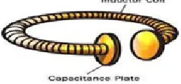
Family unit gadgets create generally little magnetic fields. Therefore, chargers hold gadgets at the separation important to initiate a present, which can just happen if the curls are near one another. Since an attractive field spreads every way, making a bigger one would squander a considerable measure of vitality. An effective approach to exchange control between loops isolated by a couple of meters is that we could expand the separation between the curls by adding resonance to the condition. A decent approach to comprehend resonance is to consider it as far as sound. A question's physical structure - like the size and state of a trumpet - decides the recurrence at which it normally vibrates. This is its resonant recurrence. It's anything but difficult to motivate articles to vibrate at their full recurrence and hard to inspire them to vibrate at different frequencies. This is the reason playing a trumpet can make an adjacent trumpet start to vibrate. The two trumpets have the same resounding recurrence. Enlistment can occur little distinctively if the electromagnetic fields around the loops resound at a similar recurrence. The hypothesis utilizes a bended curl of wire as an inductor. A capacitance plate, which can hold a charge, joins to each finish of the loop as appeared in Figure 1. As power goes through this curl, the loop starts to reverberate. Its thunderous recurrence is a result of the inductance of the curl and the capacitance of the plates.

Figure 1. Curl with Capacitance Plate.

exponential rot with separate. On the off chance that a legitimate full waveguide is brought close to the transmitter, the evanescent waves can enable the vitality to burrow (particularly transient wave coupling, what might as well be called burrowing to the power drawing waveguide, where they can be corrected into DC control. Since the electromagnetic waves would burrow, they would not proliferate through the air to be ingested or scattered, and would not disturb electronic gadgets. For whatever length of time that the two loops are out of scope of each other, nothing will happen, since the fields around the curls aren't sufficiently solid to influence much around them. So also, if the two curls reverberate at various frequencies, nothing will happen. Be that as it may, if two resounding loops with a similar recurrence get inside a couple of meters of each other, surges of vitality move from the transmitting curl to the accepting loop. As per the hypothesis, one loop can even send power to a few getting curls, as long as they all resound at an indistinguishable recurrence from appeared in Figure 2. The specialists have named this non-radiative vitality exchange since it includes stationary fields around the curls as opposed to fields that spread every way.

Figure 2. Power Transmission.

As indicated by the hypothesis, one loop can energize any gadget that is in go, as long as the curls have the same full recurrence. "Full inductive coupling" has enter suggestions in taking care of the two principle issues related with non-resonant inductive coupling and electromagnetic radiation, one of which is caused by the other; separation and productivity. Electromagnetic enlistment chips away at the rule of an essential curl producing a transcendently attractive field and an optional loop being inside that field so a current is actuated inside its loops. This causes the moderately short range because of the measure of energy required to create an electromagnetic field. Over more noteworthy separations the non-resonant enlistment strategy is wasteful and squanders a great part of the transmitted vitality just to expand. This is the place the resonance comes in and helps productivity significantly by "burrowing" the magnetic field to a collector loop that resounds at a similar recurrence. Not at all like the different layer optional of a non-resonant transformer, such accepting loops are single layer solenoids with firmly divided capacitor plates on each end, which in mix enable the curl to be tuned to the transmitter recurrence in this manner dispensing with the wide vitality squandering "wave issue" and permitting the vitality used to concentrate in on a particular recurrence expanding the range.

Remote Sensor Network Model

Manuscript characterizes the system model and remote radio model and both are used at the time of simulation.

System Model

Expect n sensor hubs are arbitrarily and consistently appropriated for the detecting ground R and the sensor organize the accompanying arrangements:

a. The system is a fixed minimally conveyed arrange. Two directional geographic places are used to convey the n number of sensors.

b. The entire hubs are coordinate with time.

c. In this one main station, which is sent at (80, 80) location.

e. This contains three sorts of hubs typical, progress, super hubs. Progress, super hubs are outfitted with more array vitality than ordinary hub.

f. These hubs consistently dispersed with the area R and it is not versatile.

Remote Radio Model

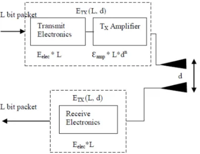
We have utilized comparable remote radio dissemination display as planned in and delineated in Figure 3. According to the radio dispersal display Signal-to-Noise Ratio (SNR) in sending a L bit data over a separation d, vitality extended by the broadcasting is given by Eq. 1 and to get this message, the broadcasting uses vitality as:

Figure 3. Remote Radio Model.

ETX = Eelec*L + εamp *L*dn (1) Where Eelec is the vitality scattered per bit. εfs and εmp on the transmitter enhancer. d is the separation between the sender and the collector. d=d0, we have d0 = √ εfs/εmp. To get a L bit message the radio uses

*

Rx L elec

E

E

Table 1. Parameters Metrics.

Description Symbol Value

Energy consumed by the amplifier to transmit at ashorter distance εfs 10nJ/bit/m2

Energy consumed by the amplifier to transmit at alonger distance εmp 0.0013pJ/bit/m4

Energy consumed in the electronics circuit to transmitor receive the

signal Eelec 50 nJ/bit

Energy for data aggregation EDA 5 nJ/bit/Signal

Message Size L 4000

Algorithm for SNLP and Simulation

Choice of sensor leader and states relies upon both the vitality stage of every sensor and separation. The calculation has the accompanying advances:

1: The area of main station settled at (80, 80) and sensors are perused from the record. It have the information for sensors position, sensors id and set the underlying vitality esteem for every sensor hub.

2: Sensor hubs systems are separated into three classifications of the sensor, for example, advance hubs, super hubs and typical hubs.

3: At any outcome, every sensor remains in one form out of the three type like Active, Idle and deciding state.

5: At this point when sensors hubs are in a choosing state with extend r, at that point it will change their state into: dynamic and sit.

6: For every sensor

i. In DLAPSH, the weight adjusting calculation is utilized to keep however many sensors living as would be prudent and after that let them expire at the same time. Dynamic state with detecting range r, if area R which isn't secured by another dynamic or choosing sensors. Sit without moving status when a sensor is abused contrasted with its side hubs or when a sensor diminishes its range to 0. This procedure blocks after all sensors settle on a choice.

ii. In PPDPSH, endeavors to limit the vitality utilization for little vitality sensors and amplify vitality utilization for upper vitality sensors. Every sensor chooses which sensor is leader hub of by utilizing the maximal lifespan of all the sensor of its side hubs. In the wake of building this conclusion, every sensor chooses to end up noticeably dynamic with extend (r ≤ most extreme detecting extent) or chooses to rest. This procedure stops after all sensors settle on a choice.

7: The choice of the considerable number of states to be dynamic or sit still state is chosen by sensors and every sensor will remain in that state for a predefined timeframe called, rearrange time, or upto that time when leader sensor expends its vitality supply and will kick the bucket. Here reminder is utilized for cautioning all sensors and afterward they change their state back to the choosing state with their most extreme detecting extent and rehash the procedure from stage 6.

8: The Simulation is rehashed until the point that vitality stage of all sensors achieves 0. 9: At that point, the procedure completes and the lifespan of the remote sensor systems is out.

System Setup

For the recreation reason, we made a static system of sensors in a 150m x 150m territory. The flexible options are: S, number of sensor hubs. We fluctuate this from 40 to 200. There is one base station at area (80, 80). P detecting ranges r1, r2,...,rP. We shift P this from 1 to 6 and every sensor P = 6 detecting ranges with values ten, twenty, thirty, forty, fifty and sixty. The underlying vitality of every sensor hub is 0.5 J. In this manuscript, the vitality demonstrate is characterized as the systems of all hubs having diverse starting vitality and sensor hubs are furnished with more vitality assets than the ordinary sensor hubs. Let m be the division of the aggregate number of hubs n, and mo is the level of the aggregate number of hubs m which are furnished with β times more vitality than the ordinary hubs, we call these hubs as super hubs. The rest n*m*(1-m0) nodes are outfitted with α times more vitality than the typical hubs; we allude to these hubs as cutting edge hubs and remaining n*(1-m) as ordinary hubs.

We assume that all hubs are appropriated consistently finished the sensor area R. Assume E0 is the underlying vitality of every ordinary hub. The vitality of every super hub is then (1+β) and each propelled hub is then E0 (1+α). The aggregate starting Energy is

E=n*(1-m)*E0 +n*m (1-m0)*E0*(1+ α) +n*m*m0*E0*(1+ β) (3)

E=n*E0*(1+m*(α+m0* β)) (4) is the aggregate starting vitality of the new heterogeneous system.

Results

Power Proficient Data Gathering Protocol (PPDPSH)

The accompanying sections examine the reenactment comes about for PPDPSH and their lifespan correlations with various customizable detecting ranges accounted for.

Option 1: α =2, β =1, m=0.3, m0=0.6

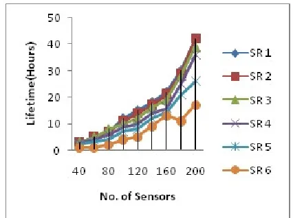
Figure 4 shows the lifespan for sensor hubs if there should be an occurrence of heterogeneous hubs and distinctive customizable detecting ranges. It is watched that when the detecting range is differed from one to four there is noteworthy augmentation in lifespan of the system while detecting range for other is little bit different. Manuscript demonstrated that for 200 quantities of sensors the lifespan got if there should be an occurrence of PPDPSH is [18.70, 28.40, 33.89, 39.22, 42.41, and 42.80] separately if there should be an occurrence of detecting scopes of one to six.

Figure 4. Lifespan vs No. of nodes (Different Sensor Range).

Option 2: α =1, β =2, m=0.3, m0=0.6

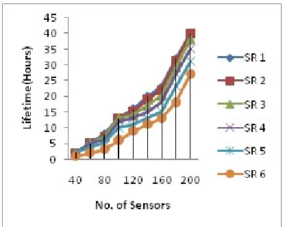
Make sense of Figure 5 focuses on the lifespan of sensor organizes if there should be an occurrence of heterogeneous hubs and diverse customizable detecting ranges. It is reasoned that when the detecting range is shifted from one to four. Change in lifespan of the system while detecting range for other is little bit different. Manuscript demonstrated that for 200 quantities of sensors the lifespan acquired if there should be an occurrence of PPDPSH is [17.87, 26.99, 32.78, 36.56, 38.83, and 38.67] individually if there should arise an occurrence of detecting scopes of one to six.

Figure 5. Lifespan vs No. of nodes.

Data gathering Load Adjustment Protocol (DLAPSH)

Option 1: α =2, β =1, m=0.3, m0=0.6

Figure 6 give data about the lifespan of sensor arranges if there should be an occurrence of heterogeneous sensor hubs and diverse customizable detecting ranges. It is continuous watching that when the detecting range is differed from one to four there is critical change in lifespan of the remote system while detecting range for other is little bit different. Manuscript demonstrated that for 200 quantities of sensors the lifespan acquired if there should arise an occurrence of DLAPSH is [19.98, 29.86, 35.78, 39.94, 42.90, and 42.92] individually in the event of detecting scopes of one to six.

Figure 6. Lifespan vs No. of nodes (different sensor ranges).

Option 2: α =1, β =2, m=0.3, m0=0.6

Figure 7 shows the lifespan for sensor hubs if there should be an occurrence of heterogeneous hubs and distinctive movable detecting ranges. It gives the reason that when the detecting range is shifted from one to four there is noteworthy augmentation in lifespan of the system while detecting range for other is little bit different. Results demonstrated that for 200 quantities of sensors the lifespan got if there should be an occurrence of DLAPSH is [18.75, 26.94, 32.76, 36.68, 39.87, and 39.84] separately if there should arise an occurrence of detecting scopes of one to six.

Figure 7. Lifespan vs No. of nodes.

Conclusion

DLAPSH function admirably in expanding the system lifespan and diminishing the vitality utilization to transmit information in reproduction. In every one of the options for PPDPSH and DLAPSH conventions, the lifespan of sensor systems demonstrates an addition [19 to 43; 18 to 36; 21 to 47] and [20 to 47; 19 to 37; 20 to 45] hours for detecting range one to six separately. With the help of Wireless power transfer the power problem of wireless sensor network reduce significantly.

References

[1] D. Kumar, T. S. Aseri, R. B. Patel “EEHC: Energy efficient heterogeneous clustered scheme for wireless sensor networks”, Inter J of Comp. Comm., Elsevier, 2008, 32(4): 662-667, March 2009.

[2] W. Heinzelman, A. Chandrakasan and H. Balakrishnan. “An Application-Specific Protocol Architecture for Wireless Microsensor Networks," IEEE Transactions on Wireless Communications, Vol. 1, No. 4, 660-670, October 2002.

[3] S. Lindsey, C.S. Raghavendra, PEGASIS: power efficient gathering in sensor information systems, in: Proceedings of the IEEE Aerospace Conference, Big Sky, Montana, March 2002, Vol.3, pp. 3-1125- 3-113.

[4] SH. Lee, JJ. Yoo and TC. Chuan, “Distance-based Energy Efficient Clustering for Wireless Sensor Networks”, Proc. of the 29th IEEE Int’l Conf. on Local Computer Networks (LCN’04)

[5] O. Younis and S. Fahmy, “Distributed Clustering in Adhoc Sensor Networks: A Hybrid, Energy-Efficient Approach”, In Proc. of IEEE INFOCOM, March 2004.

[6] J. M. Kim, S. H. Park, Y. J. Han, and T. M. Chung, “CHEF: Cluster Head Election mechansim using Fuzzy logic in Wireless Sensor Networks”, Proc. of ICACT, 654- 659, Feb. 2008.

[7] M. Bhardwaj. Selection of Efficient Relay for Energy-Efficient Cooperative Ad Hoc Networks. Amer J of Netw and Comm. Special Issue: Ad Hoc Networks. Vol. 4, No. 3-1, 2015, pp. 5-11. doi: 10.11648/j.ajnc.s.2015040301.12

[8] M. Bhardwaj, Enhance life Time of Mobile Ad hoc Network using WiTriCity and Backpressure Technique, 1877-0509 © 2015 The Authors. Published by Elsevier B.V. This is an open access article under the CC BY-NC-ND license, doi: 10.1016/j.procs.2015.07.447.

[9] M. Bhardwaj, A. Ahlawat, Reduce Energy Consumption in Ad Hoc Network with Wireless Power Transfer Concept. Inter J of Cont Theor and App 2017; 10: 125-13.

[10] M. Bhardwaj, Selection of Efficient Relay for Energy-Efficient Cooperative Ad Hoc Networks. American J of Netw and Comm 2015; 4(3), 5-11.

[11] J. Kim, J. Jang, AODV based Energy Efficient Routing Protocol for Maximum Lifespan in MANET. In: IEEE 2006, Conference on Telecommunications; 19-25 Feb 2006; Guadelope, French Caribbean: IEEE. pp. 1-212.

[12] L. Guo, Y. Liu, T. Huizhu Ma, Jiang, Energy Efficient on–demand MultipathRouting Protocol for Multi-hop AdHoc Networks. In: IEEE 2008, Symposium on Spread Spectrum Techniques and Applications; 25-28 Aug 2008; Bologna, Italy: IEEE. pp. 1-820.

[13] V. Kanakaris, D. Ndzi and D. Azzi, Ad-hocnetworks energy consumption: A review of the ad hoc routing protocols. J of Engg and Techn 2010; 3, 162-167.

[14] M. Tamilarasi, T. G. Palanivelu, Integrated Energy-Aware Mechanism for MANETs usingon demand Routing.Intern J of Compand Inform Engg 2008; 2(2), 253-257.

2005 International Workshop on Wireless Ad hoc Networks; 23-26 may 2005; King’s College London, London: IEEE.

[16] R. C. Shah, J. M. Rabaey, Energy aware routing for low energy ad hoc sensor networks. In: IEEE 2002 Wireless Communications and Networking; 17-21 March 2002; Orlando, FL, USA: IEEE. pp. 1-931.

[17] B. K. Saraswat, M. Bhardwaj, A. Pathak, Optimum Experimental Results of AODV, DSDV & DSR Routing Protocol in Grid Environment. In: Elsevier 2015 Procedia computer science, Conference on Recent Trends in Computing; 12-13 March 2015; Ghaziabad, India: Elsevier. pp. 1342-1350.

[18] M. Bhardwaj, Enhance Life Time of Mobile Ad-hoc Network Using WiTriCity and Backpressure Technique. In: Elsevier 2015, Procedia computer science, Conference on Recent Trends in Computing; 12-13 March 2015; Ghaziabad, India: Elsevier. pp. 1342-1350.

[19] M. Bhardwaj, A. Singh, Power Management of Ad Hoc Routing Protocols Using Mobility Impact and Magnetic Resonance. Advan in Networks 2015; 3(3), 27-33.

[20] M. Bhardwaj, A. Bansal, Energy Conservation in Mobile Ad Hoc Network Using Energy Efficient Scheme and Magnetic Resonance. Advan in Networks 2015; 3(3), 34-39.

[21] M. Veerayya, V. Sharma, A. Karandikar, SQ-AODV: A novel energy aware stability based routing protocol for enhanced QOS in wireless ad-hoc networks. In: IEEE 2008 Military Communication Conference (MILCOM); 16-19 Nov 2008; San Diego, California, USA: IEEE. pp. 4-165.

[22] K.T. Sikamani, P. K. Kumaresan, M. Kannan, R. Madhusudhanan, Simple Packet Forwarding and Loss Reduction for Improving Energy Efficient Routing Protocols in Mobile Ad-Hoc Networks. Euro J of Sci Resea 2009.

[23] H. Huang, G. Hu, F. Yu, A Routing Algorithm Based on Cross-layer Power Control in Wireless Ad Hoc Networks. In: IEEE2010 Communications and Networking in China (CHINACOM); 25-27 Aug 2010; Beijing, China: IEEE.

[24] R. Ghanbarzadeh, R. M. Meybodi, Reducing message overhead of AODV routing protocol in urban area by using link availability prediction. In: IEEE 2010Conference on Computer Research and Development; 7-10 May 2010; Kuala Lumpur, Malaysia: IEEE. pp. 3-898.

[25] A. H. Mohammed, M. RaviSankar, V. Kumar, N. Lovanjaneyulu, R. Srinivasa, Energy Conservation Techniques in Ad hoc Networks. Intern J of Comp Sci and Inform Techno 2011; 2, 1182-1186.

[26] C. E. Perkins, E. M. Royer & S. R. Das, Ad Hoc On-Demand Distance Vector (AODV) Routing. In: IEEE 1999 Workshop on Mobile Computing System and Applications; 1999; New Orleans LA, USA: IEEE. pp. 90-100.