2017 2nd International Conference on Software, Multimedia and Communication Engineering (SMCE 2017) ISBN: 978-1-60595-458-5
Dual Random Projection for Linear Support Vector Machine
Xi XI
*, Feng-qin ZHANG
and Xiao-qing LI
Institute of Information and Navigation, Air Force Engineering University, Xi’an 710077, China *Corresponding author
Keywords: Machine learning, Support Vector Machine (SVM), Random projection, Dimensionality reduction.
Abstract. Support Vector Machine (SVM) is a popular machine learning methods in the field of data analysis. The Random Projections (RP) method can solve the problem of dimensionality reduction of high-dimensional data quickly and effectively to reduce the computational cost of the related optimization problem and is widely used in the SVM method. However, the large-scale SVM has the problem of reduced classification accuracy after dimension reduction by random projection feature. Therefore, we propose a linear kernel support vector machine based on dual-random projection (drp-LSVM) for large-scale classification problem, which combines the duality recovery theory. In this paper, we analyze the geometric properties of drp-LSVM, and prove that while dividing the geometric advantage of support vector machine based on random projection (rp-LSVM), the division of hyperplane is closer to that obtained by all data training Original classifier. The experimental results show that the drp-LSVM can reduce the classification error and improve the training precision, and the performance evaluation is closer to the classifier trained with the original data while inheriting the advantages of rp-LSVM.
Introduction
Support Vector Machine (SVM) [1] has the advantage of dealing with small sample, non-linear data, and high-dimensional pattern recognition. It can in a certain extent to avoid "dimension disaster". So SVM-based classifier is widely used in dealing with high-dimensional data classification problem, and at the same time, the feature reduction method applied to large-scale SVM has become a hotspot. In recent years, stochastic approximation algorithms have been widely used in large-scale machine learning, and the Random Projections (RP) method can quickly and effectively solve the dimensionality problem of high-dimensional data in order to reduce the computational cost of related optimization problems. Random projection is a method of reducing the dimension by controlling the precision, keeping the distance between the two samples in pairs, and therefore belonging to the distance-based method. Since SVM is also based on the distance learning method, it can be used to reduce the dimensionality of random projection. From 2007 to 2009, Krishnan et al. [2] and Jethava et al. [3] demonstrated that SVM based on Gaussian random projection can obtain correlation errors similar to the original problem, and the training time is related to the projection matrix and the input matrix. Paul et al. [4] demonstrated that the use of random projection data after SVM training can maintain the geometric properties of the feature space while maintaining the maximum interval of the classifier and the minimum closure of the geometric properties of the closed ball, to maintain the original pan And theoretically proves that the linear kernel SVM based on random projection (rp-LSVM) training time is linearly related to the number of non-zero data input.
to the rp-LSVM, and propose a linear kernel SVM based on dual random projection (drp-LSVM), which solves the advantages of rp-LSVM Accuracy of the problem. The theoretical analysis shows that drp-LSVM is geometrically closer to the original classifier obtained by all data training than rp-LSVM. It is proved that the maximum interval of drp-LSVM hyperplane and minimum closed ball keep the geometric properties similar to rp-LSVM; also to ensure that the original space similar to the generalization ability. The experimental results show that the drp-LSVM can reduce the training error and improve the training precision while the performance of the rp-LSVM is improved. The performance evaluation of the training result is closer to the classifier trained with the original data.
Definitions and Notations
Notation and SVM Basics
Let D
x ,i yi
, i1 2, ,...,n be a set of training examples, where xiRd and yi
1 1,
is Class tag.For the linearly separable data, the most basic idea of the SVM learning problem is to find a division of the hyperplane with the largest interval in the sample space based on the training set D [6]. Into a convex quadratic programming problem is:
2
1 min
2
w w (1)
s.t. yiw x, i 1, i
1,...,n
(2)This is the basic form of SVM, where w is the normal vector for dividing the hyperplane. When the soft interval and regularization ideas are added and the kernel function is a linear kernel, the corresponding Lagrange dual problem is:
n
T
R
1 1 1
1 max
2
n n n
i i j i j
i i j
y y x xi j (3)
s.t.
1
0
n
i i
i y
(4)Here, is the Lagrange operator; C is constant.
Let sample data set be within the sphere with semi diameter of R and the let the distance sum (SVM interval) of support vector to the hyperplane be , then the of the assuming set is O R
2 2
, in which way the generalization errors can be estimated.Random Projection Method
The Random Projection algorithm[8][9] is extensive used in Classification, Clustering, Regression,
Ensemble Learning and other fields. Let n k
:R R
P is a random projection (RP), ARk d is a
standard random orthogonal matrix. From Johnson-Lindenstrauss lemma[7], we can know that the A
can maps the set of arbitrary m points in a d-dimensional space to a k-dimensional space (k d). RP not only can keep the nature of the distance, but also can retain the characteristics of the original data with high probability. Here we explain that although the random projection matrix is divided into a variety of, but the random projection matrix referred to in this paper are Gaussian projection matrix.
Lemma 1.1: Let
0 1, , n and m is a positive integer and satisfies this condition:
2 3
1m4 /2 /3 ln n.
2
2
21 u v P u P v 1 u v (5)
Theorem 1: Through the standard Gaussian matrix random projection, we get xRn fromαRd, and:
2 2 2
2 2 2
2 3
1 1
1 2 4
P
exp d
x α x
(6)
Lemma 1.2[5]: Let0 1 2,
0 1, , VRm n is an arbitrary positive definite matrix, m rR
A is
gaussian random matrix, and rO n
2log n
, Then at least the probability of 1 has thefollowing inequality holds T T T
V V V AA V .
Proposed Method
Drp-LSVM
The support vector machine problem can be converted to convex quadratic programming problem, so, by using Lagrange multiplier method, the dual problem can be solved. Comparing to the method raised by Zhang[5], which showed that in dual random projection algorithm, the conjugated dual variables in the low dimensional optimization problem are brought to the original problem to regain the optimal solution, the Lagrange multiplier solved in the low dimensional place can be brought to the calculation of the original hyperplane in order to get the presumptive optimal hyperplane.
Let X be the input data matrix, where each row is an input vector T
i
x and each column is a feature,
we can get the optimal solution vector
1 2
* * * *
m
, ,...,
α by solving the LSVM Lagrange dual
problem as follow:
T T1
1 2
m * * * *
i i
W α α YXX Yα (7)
A is a Gaussian projection matrix that satisfies Lemma 2,
1 2
~ ~ ~ ~
* * * *
m
( ; ;...; )
is the Lagrange
optimal solution vector obtained after random projection, then:
T T T
1
1 2
~ ~ ~
m ~
* * *
i W
~ *
α α α YXAA X Y α (8)
The relationship between the optimal solution of the original problem and the optimal dual solution are:
T T
T T
* *
~ ~
* *
w α YX
w α YXA
(9)
2 2
1
2 2
1
m
* *
i i
~ m ~
* *
i i
ww
(10)
Then we can get the optimal intervals:
1 2
* *
1 2
~* w~* (12)
We extend the Lagrange optimal solution vector of low dimensional space into the original
problem, the optimal hyperplane is T T
~
* *
w α YX , and the geometric interval is 2 1
* *
w .
Geometric Properties
Let the original problem have the optimal solution *
w , drp-SVM have the optimal solution *
w , then:
1
* *
*
w w
w
(13)
Prove as follows:
LetEV VT V AA VT T , when the problem (7) and (8) after SVD decomposition, we can get:
T T T T T T1
T T T T
1
1 1
2 2
1 2
m
* * * * * *
i i
~ m ~ ~ ~
~
* * * *
i
W
W
α α YUΣV AA VΣU Yα α YUΣEΣU Yα
α α α YUΣV AA VΣU Y
(14)
And then we get:
1 T T T T2
~ ~ ~ ~
* * * * * *
W W
α α α α YUΣV AA VΣU Y α α (15)
And by the Lagrange dual function of the concave we can get:
T
~ ~ ~
T T T
T
~ ~
~
T T T T T
1 2
* * * * *
* * * * *
W
W
α α α YUΣV AA VΣU Y α α
α α α YUΣV AA VΣU Y YUΣV VΣU Y α α
(16)
That is:
T T
~ ~ ~
T T T T
* * * * * * *
α α YUΣEΣU Yα α α YUΣV AA VΣU Y α α (17)
By lemma2 we get
1
2 2 * * *
w w w (18)
When optimal solution of the lower space is transformed into high dimensional space, there is
T
~
* *
w AA w (19)
Then
2 1 2 2
~
* * * *
w w w w (20)
~ ~ ~ ~ ~
T T T T T T
1
1 1
2 2
m
* * * * * *
i
W ( )
α α α YUΣV AA VΣU Y α α YUΣEΣU Y α (21)
Then,
~ ~ ~ ~ ~
T T T 2
2 2
1 1
2 2
* * * * * *
W(α ) W( α ) α YUΣEΣU Y α W(α ) E α YX (22) We get:
T 2 *T 2
2 2
T T T T T
T T
T 2
2 2
~ ~
*
~ ~ ~ ~
* * * *
~ ~
* *
~ *
| |
| |
| |
α YXA α YX
α YXAA X Y α α YXX Y α
α YUΣ E ΣU Y α
E α YX
(23)
Then we can get:
T 22 2 2
1
1 2
~ ~
* * *
W α W α E E α YXA (24)
We have
22
1 2
* *
W α w , 22
1 2
~ *
W
~ *
α w and then from (18) we get:
2 2 2
2 2 2 1 2 2
~ ~
* * *
w w E E w (25)
From (19) we can get
2 2
2 1 1 2 2
~ *
*
w E w (26)
Combining (20) and (26), we get
2 2
2 1 2 2 2
* *
w E w (27)
That is:
2 2
2
1 2
* *
E (28)
From lemma 2, we get:
2 2
2 2
1 2
1 1
* *
~
* *
, (29)
Likewise, SVD and Lemma 2 can be used to demonstrate that the properties of the Minimum Closed Ball (MEB) are as follows. Since the LSVM's MEB's Lagrange dual issue is:
T T T T
T1 1 0
max diag
s.t. ,
α XX α XX α
α α (30)
Let the ball radius isR, the center of the ball vector isxc, then:
2 T T T T
1
mc i i
i x
x (32)
After random projection:
2 T T T T T T
~ ~ ~ ~
R α diag XAA X α XAA X α (33)
After dual recovery:
2 T T T T
~ ~ ~
R α diag XX α XX α (34)
Combined with lemma 2, it easy to push that:
2 2 2
2 2
1 1
~
R R R
R R
(35)
From the above theoretical analysis, we can get that the hyperplane and the radius of MEB of the drp-LSVM is similar to the rp-LSVM, and it also maintains the correlation error with the original space, maintaining the generalization performance similar to that of the original space.
Experiment
The experimental environment is 2.6 GHz Intel Core i5 processor, 8GB memory, operating system for linux, development tools for Python, Java. The experimental data is from libsvm Data [9]. Experiment 1 is based on the liblinear [10] library for drp-SVM correlation performance test, and the parameter is set as the default parameter. Experiment 2 tests the performance of the drp-SVM based on the improved SMO algorithm. The data sets D1 and D2 are gisette_scale [11], rcv1.binary [12], respectively. D1 contains the training sample 6000, the test sample 1000, the sample dimension is 5000 to meet the medium-scale data volume and dimension characteristics; D2 with training samples 202421, test sample 677399, dimension 47236, to meet the large-scale high-dimensional data characteristics. In order to ensure the accuracy and credibility of the experiment, the relevant experiments were repeated 5 times, and the final experimental data were averaged.
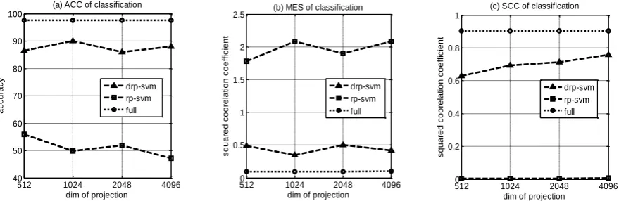
For the medium-scale data set D1, in order to check the effect of the classifier, taking the data set dimension of 5000, we took four different projection dimensions 512,1024,2048,4096, respectively, in a variety of target dimensions drp-SVM, rp-SVM and the original classifier (that is, with all the data training out of the support vector machine, shown in the full full) related evaluation parameters. Figure 1 (a), Figure 1 (b) and Figure 1 (c) show the accuracy (ACC) ,mean square error (MSE) and square correlation coefficient (SCC)of the three classifiers in different dimensions.
512 1024 2048 4096
40 50 60 70 80 90 100
(a) ACC of classification
dim of projection
a
c
c
u
ra
c
y
drp-svm rp-svm full
512 1024 2048 4096
0 0.5 1 1.5 2
2.5 (b) MES of classification
dim of projection
s
q
u
a
re
d
c
o
o
re
la
ti
o
n
c
o
e
ff
ic
ie
n
t
drp-svm rp-svm full
5120 1024 2048 4096
0.2 0.4 0.6 0.8 1
(c) SCC of classification
s
q
u
a
re
d
c
o
o
re
la
ti
o
n
c
o
e
ff
ic
ie
n
t
[image:6.595.83.523.628.771.2]From Figure 1, we can get that compared to rp-SVM, drp-SVM of the training indicators are closer to all the training data obtained by the original classifier.
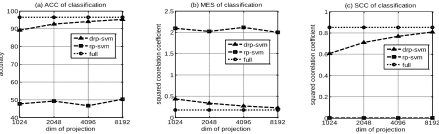
For the larger-scale data set D2, considered the dimension of the data set 47236, we took four different projection dimensions 1024,2048,4096,8192, in a variety of target dimensions were calculated drp-SVM, rp-SVM And the original classifier (that is, with all the data trained out of the support vector machine, shown in the full full) related evaluation parameters. Figure 2 (a), (b) and (c) are the relationship between accuracy (ACC), mean square error (MSE) and square correlation coefficient (SCC) of the three classifiers in different dimensions.
1024 2048 4096 8192 40
50 60 70 80 90 100
(a) ACC of classification
dim of projection
a
cc
u
ra
cy
drp-svm rp-svm full
10240 2048 4096 8192 0.5
1 1.5 2 2.5
(b) MES of classification
dim of projection
sq
u
a
re
d
c
o
o
re
la
tio
n
c
o
e
ffi
ci
e
n
t
drp-svm rp-svm full
10240 2048 4096 8192 0.2
0.4 0.6 0.8 1
(c) SCC of classification
dim of projection
sq
u
a
re
d
c
o
o
re
la
tio
n
c
o
e
ffi
ci
e
n
t
[image:7.595.83.522.197.331.2]drp-svm rp-svm full
Figure 2. Performance index of each classifier under different dimensions for D2.
From Figure 2, we can get that that the training index of drp-svm is better than rp-svm in the large-scale higher-level data set environment, and closer to the original classifier.
Table 1 and 2 are the statistics for the data set D1 and D2 training different classifiers in the optimal projection dimension training time (time, unit: s), the maximum interval (γ), 5 cross-check (5-fold) The accuracy and classification error rate (errorRate).
Table 1. Parameters of three classifiers trained by D1. D1 rp-svm drp-svm full time(s) 13.20 25.65 36.90
γ 0.761 1.430 1.739 5-fold 96.48 97.13 97.21
errorRate 0.1 0 0
Table 2. Parameters of three classifiers trained by D2. D2 rp-svm drp-svm full time 176.16 204.06 238.89
γ 0.0560 0.0537 0.0491
5-fold 96.63 97.19 97.37 errorRate 1.47e-6 0 0
By Table 1 and 2, we can get that, compared to rp-svm, drp-svm retained the advantage that it reduces the training time and maintain the maximum interval, and on this basis to improve the training accuracy and reduce the error.
Conclusions and Open Problems
interval super-plane and the minimum closure sphere of drp-LSVM maintain the ε-related error similar to rp-LSVM, and also ensure the generalization ability similar to that of the original space. Experiments show that the drp-LSVM is more close to the original classifier than the original linear kernel support vector machine and Gaussian projection, and the training effect and performance evaluation are not considered non-linear and other types of random projection features reduced dimension. Large-scale machine learning is still the current mainstream challenges, the random machine learning technology approach to be further in-depth study.
References
[1] Cortes C, Vapnik V. Support-vector networks[J]. Machine Learning, 1995, 20(3):273-297.
[2] Kumar K, Bhattacharyya C, Hariharan R. A Randomized Algorithm for Large Scale Support
Vector Learning[C]// Conference on Neural Information Processing Systems, Vancouver, British Columbia, Canada, December. DBLP, 2007:793-800.
[3] Jethava V, Suresh K, Bhattachryya C, et al. Randomized Algorithms for Large scale SVMs[J].
Computer Science, 2009.
[4] Paul S, Boutsidis C, Magdon-Ismail M, et al. Random Projections for Linear Support Vector
Machines[J]. ACM Transactions on Knowledge Discovery from Data, 2014, 8(4):1-25.
[5] Zhang L, Mahdavi M, Jin R, et al. Recovering the Optimal Solution by Dual Random Projection[J]. Journal of Machine Learning Research, 2012, 30:135-157.
[6] Zhou Z H. Machine Learning.[M] Beijing: Tsinghua University Press,2016:121-145
[7] Liu H, Liu R, Li S. Acceleration gesture recognition based on random projection [J]. Journal
of Computer Applications, 2015, 35(1): 189-193.
[8] Wang P, CaiS J, Liu Y. Improvement of matrix completion algorithm based on random projection [J]. Journal of Computer Applications, 2014, 34(6): 1587-1590.
[9] Chang C, Lin Lin C J. LIBSVM: A library for support vector machines[J]. Acm Transactions
on Intelligent Systems & Technology, 2011, 2(3):27.
[10] Fanr E, Chang K W, Hsieh C J, et al. LIBLINEAR: A Library for Large Linear
Classification[J]. Journal of Machine Learning Research, 2008, 9(9):1871-1874.
[11] Golub T R, Slonim D K, Tamayo P, et al. Molecular classification of cancer : class discovery and class prediction by gene expression monitoring. Science, 286(5439):531, 1999.