Methods for change point detection with additional interpretability

(1)

Methods for Change-Point Detection with

Additional Interpretability

London School of Economics and Political Sciences

Anna Louise M. M. Schr¨

oder

A thesis submitted to the Department of Statistics of the London

School of Economics for the degree of Doctor of Philosophy,

(2)

(3)

Declaration

I certify that the thesis I have presented for examination for the MPhil/PhD degree of the London School of Economics and Political Science is solely my own work other than where I have clearly indicated that it is the work of others (in which case the extent of any work carried out jointly by me and any other person is clearly identified in it). The copyright of this thesis rests with the author. Quotation from it is permitted, provided that full acknowledgement is made. This thesis may not be reproduced without my prior written consent. I warrant that this authorisation does not, to the best of my belief, infringe the rights of any third party. I declare that my thesis consists of 57,322 words.

Statement of conjoint work

I confirm that Chapter 3 was jointly co-authored with Professor Piotr Fryzlewicz and I contributed 75% of this work. I confirm that Chapter 5 was jointly co-authored with Professor Hernando Ombao and I contributed 75% of this work.

(4)

(5)

Abstract

The main purpose of this dissertation is to introduce and critically assess some novel statistical methods for change-point detection that help better understand the nature of processes underlying observable time series.

First, we advocate the use of change-point detection for local trend estimation in financial return data and propose a new approach developed to capture the oscilla-tory behaviour of financial returns around piecewise-constant trend functions. Core of the method is a data-adaptive hierarchically-ordered basis of Unbalanced Haar vectors which decomposes the piecewise-constant trend underlying observed daily returns into a binary-tree structure of one-step constant functions. We illustrate how this framework can provide a new perspective for the interpretation of change points in financial returns. Moreover, the approach yields a family of forecasting operators for financial return series which can be adjusted flexibly depending on the forecast horizon or the loss function.

Second, we discuss change-point detection under model misspecification, focus-ing in particular on normally distributed data with changfocus-ing mean and variance. We argue that ignoring the presence of changes in mean or variance when testing for changes in, respectively, variance or mean, can affect the application of statis-tical methods negatively. After illustrating the difficulties arising from this kind of model misspecification we propose a new method to address these using sequential testing on intervals with varying length and show in a simulation study how this approach compares to competitors in mixed-change situations.

(6)

(7)

Dedication

To my family - für meine Familie: meine Eltern und meine Schwester Julia, die immer für mich da waren, wenn ich Ansporn oder Rat brauchte. Und für meine lieben Großeltern, die mich inspiriert haben, diese Herausforderung zu meistern.

(8)

(9)

Acknowledgements

This work was supported by the Economic and Social Research Council grant number ES/J00070/1.

I would like to thank many people who have helped me through the completion of this dissertation. Firstly, I thank my advisor, Piotr Fryzlewicz, and Hernando Ombao at University of California, Irvine, who I had the luck to collaborate with. Both gave me excellent guidance and feedback for my research over the last years, mentored and advised me honestly and shaped my perspective on the academic world. I consider myself fortunate to have been part of the LSE Department of Statistics, which offered me a great intellectual and work environment. I want to thank especially Ian Marshall, who supported academic staff and students beyond all measure.

I am deeply grateful for my friends, who continue to impress me with their intelligence, positivity and wit. I would not be the person I am without them and this dissertation has greatly benefited from our many motivating and inspiring moments in the last years. Karin Kaiser, Maria Carvalho, Kevin K’Bidi, Anja Schanbacher and Jennifer Petzold - you make London my home. Philipp Kurbel, Karol Campa˜na, Jos´e Ram´ırez Bucheli, Alex Pucola and Hanna Hoffmann - hav-ing you in my life, no matter how far, will always be great source of my energy. Guillaume Henry, your optimism and esprit made a big difference to my life in the past two years and I am deeply grateful for them.

(10)

(11)

List of Figures

1.1 S&P500 Price Index . . . 24

1.2 EEG Recording of Epileptic Seizure at Channel T3 . . . 25

2.1 Number of Search Results of the Term ‘Change Point’ . . . 30

2.2 Binary Segmentation Algorithm . . . 49

3.1 S&P 500 Index and Model Fit . . . 63

3.2 S&P 500 Index and Simulated Sample Paths . . . 71

3.3 UHP-BS Algorithm . . . 78

3.4 Daily closing values of GE, GBP-USD and WTI . . . 89

3.5 Cumulative Returns of Equity Indices . . . 100

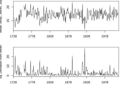
4.1 Temperature in July in Berlin . . . 109

4.2 S&P500 Price Index, 2006-2008 . . . 110

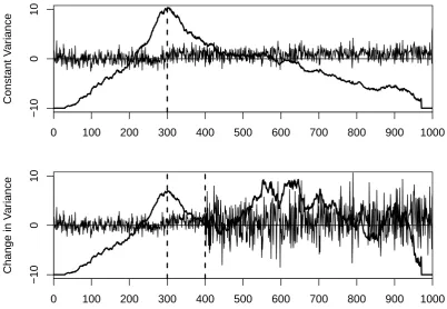
4.3 Illustration of Change-in-Mean Test Statistic . . . 121

4.4 Illustration of Change-in-Variance Test Statistic . . . 122

4.5 Illustration of Change-in-Variance Test Statistic . . . 123

4.6 Illustration of Change-in-Mean-and-Variance, All Test Statistics . . 125

(18)

4.7 Illustration of Sequential Testing Approach . . . 128

5.1 Partitioning of {1, . . . , T∗} into nonoverlapping intervals . . . 164

5.2 FreSpeD algorithm . . . 168

5.3 Realizations of processes from the simulation study . . . 174

5.4 Estimated time-varying autospectrum of the VAR(2) process . . . . 175

5.5 EEG 10-20 Scalp Topography . . . 183

5.6 EEG Recording of Epileptic Seizure at Channel F3 . . . 184

5.7 Cumulative Sum of Detected Change Points . . . 185

5.8 Change Points in the Autospectra of Channels T3 and T5 . . . 186

5.9 Preictal Changes at all Autospectra and Cross-Coherences . . . 189

B.1 Illustration of Change-in-Variance, All Test Statistics . . . 206

(19)

List of Tables

3.1 Simulation Results for VariousVηi and C . . . 87

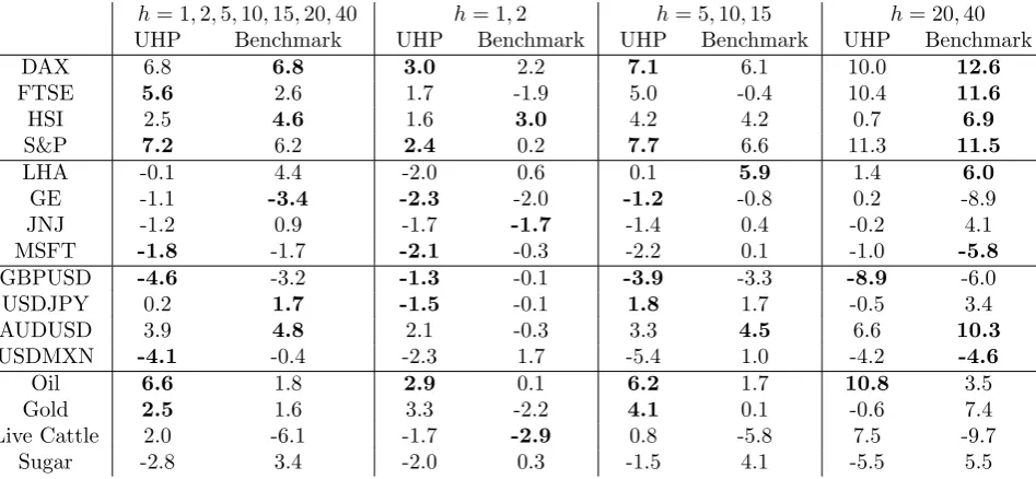
3.2 Relative Success Ratio in Percent . . . 93

3.3 Relative Success Ratio During Times of Strong Movements . . . 94

3.4 Relative Success Ratio in Percent in the Out-of-Sample Test . . . . 95

4.1 Parameter Settings for the Simulation Study . . . 135

4.2 Results for Sparse Change-Point Settings: N ={3,6} . . . 141

4.3 Results for Sparse Change-Point Settings: N ={9,12} . . . 142

5.1 Results for N = 1, D= 2 . . . 178

5.2 Results for N = 5, D= 2 . . . 178

5.3 Results for N = 1, D= 20 . . . 179

5.4 Results for N = 5, D= 20 . . . 179

5.5 Frequency-Specific Proportion of Change Points and Change Mag-nitude . . . 187

A.1 Data Series Used in the Empirical Evaluation . . . 198

A.2 Number of Forecasts of the Out-of-Sample Analysis . . . 198

(20)

A.3 Optimal in-Sample Parameter in our Model . . . 199

A.4 Optimal in-Sample Parameter in the Benchmark Model . . . 199

A.5 Number of Forecasts, Out-of-Sample Analysis with Two-Year Window200

A.6 Relative Success Ratio, Out-of-Sample Test With Two-Year Window 201

A.7 Optimal in-Sample Parameter in Our Model, Two-Year Window . . 202

A.8 Optimal in-Sample Parameter in the Benchmark Model, Two-Year Window . . . 203

C.1 Simulation Results for Varying Interval Length ν, withD= 2, N = 1 223

C.2 Simulation Results for Varying Interval Length ν, withD= 2, N = 5 224

C.3 Simulation Results for Varying Interval Lengthν, withD= 20,N = 1225

C.4 Simulation Results for Varying Interval Lengthν, withD= 20,N = 5226

(21)

Chapter 1

Introduction

The systematic understanding of our past has been in the focus of scientific research since its inception: it allows us to draw conclusions which affect future behaviour. Driven by the desire to grasp the unobservable structure underlying evolutionary time series, an increasing systematization of recorded measurements can be ob-served throughout history in a variety of areas - from environmental data such as temperature and rainfall, via socioeconomic measures of health, poverty and demo-graphic trends, to the increasingly precise measurement of time itself. Over the last century, digitalisation and technological advances in data management and stor-age have enabled scientists to systematically analyse evolution in such time series recordings with the general goal of better understanding unobserved underlying processes.

Many evolutionary processes, albeit not all, can be viewed as undergoing occa-sional, sudden transitions (Brodsky and Darkhovsky, 2013). For example, economists and policy makers classify the state of an economy into recession and recovery and are interested in identifying points in time when a transition between these states can be attested to decide on the appropriate policy measures at any such time (Diebold and Rudebusch, 1996). Similarly, in the field of seismology, researchers are concerned with identifying earthquake predictors by monitoring velocity changes in

(22)

seismic waves (Ogata, 2005). Medical doctors are monitoring physiological time se-ries to identify sudden abnormalities that may relate to a medical condition (B´elisle et al., 1998; Strens et al., 2003). From a statistical point of view, if the process underlying such a time series has a time-invariant nature between any two neigh-bouring points of transition, it can be described as piecewise-stationary process. The estimation of the number and location of time points where a transition takes place is subject of this work and will be referred to as change-point detection or time-series segmentation. Moreover, we show how certain designs of change-point detection procedures can provide insights in the data beyond change-point locali-sation.

The main purpose of this thesis is to introduce and critically assess some novel statistical methods for change-point detection that help better understand the na-ture of processes underlying observable time series. While these methods can be used in a range of different applications, they share the objective of detecting sud-den changes in piecewise-stationary time series to segment these data-adaptively into approximately stationary intervals of varying length. The ultimate goal of this work is to fill some gaps in the change-point literature and to add to the in-terpretability of certain types of observed time series, thereby allowing for a more insightful analysis and meaningful interpretation of data. Prior to our review of existing literature we illustrate the usefulness of change-point estimation by means of a few real-world applications.

(23)

23

analysis of time series data to a new stage. Data recordings from, to name a few, climate (Reeves et al., 2007; Naveau et al., 2014), speech (Chen and Gopalakr-ishnan, 1998; Zhang and Hansen, 2008), financial markets (Andreou and Ghysels, 2002; Christoffersen and Diebold, 2006), physiological processes (B´elisle et al., 1998; Strens et al., 2003), internet traffic (Kwon et al., 2006; Kim and Reddy, 2008) or astronomy (Friedman, 1996; Scargle et al., 2013) have increased in quantity and quality, giving researchers room for critical reassessment and possible enhancement of existing methods and development of new tools to analyse, understand and in-terpret this data.

(24)

Time

S&P 500 Inde

x Le

v

el

1990 1995 2000 2005 2010

500

1000

1500

1000

Figure 1.1: S&P500 Price Index, end-of-day level, daily observations between Jan-uary 1990 and June 2013

(25)

25

Time

1 2 3 4 5 6 7 8 min

−400

0

400

Figure 1.2: Recording before and during a spontaneous epileptic seizure via elec-troencephalogram. Bipolar electrode measuring electrical activity at the left-temporal channel (T3, located approximately above the left ear)

often estimated by the physician via eye-balling, while automated methods can be valuable tools for verification of such heuristic findings (Tzallas et al., 2012).

We now briefly lay out the structure of this thesis and discuss the contribution of each chapter.

Chapter 2 provides a systematic overview of the existing literature on change-point analysis and various subclasses of the topic. It introduces the reader to the relevant elementary concepts and foundations on which we build in the following chapters.

(26)

aver-age return between the most recent estimated change point and the current time. The contribution of this work goes beyond advocating change-point detection to estimate local trends in financial returns. Our main objective is to propose an alternative approach to statistical time series analysis, whereby the time series is spanned by an orthonormal oscillatory basis induced by change points in the se-ries’ conditional mean value. In this context, the representation basis is assumed to be unknown and needs to be estimated data-adaptively using a change-point detection procedure. Our approach yields a family of forecasting operators for the financial return series, parameterised by a single threshold parameter, which can be adjusted flexibly depending on forecast horizon or loss function.

Chapter 4 discusses a question related to that of Chapter 3: how to detect possibly many change points in a time series when changes can take place in the series’ conditional mean, variance or both quantities simultaneously. This more general problem of estimating number, location and type of change points has not received much attention in the literature. It comes with a number of challenges which we address using a sequential testing method. Our core contributions are to systematically describe the difficulties for change-point detection and to propose a novel method to overcome these. Moreover, we discuss computational aspects of the method and compare it to competing approaches in a simulation study.

(27)

27

characterizes energy evolution measured on the human scalp through change-point detection. In addition to discussing the features of the method and contrasting it with existing approaches, we analyse and interpret the method’s output in the application to the seizure data set which is partly depicted in Figure 1.2.

Chapter 6 concludes.

(28)

(29)

Chapter 2

Background and Related Work

2.1

Piecewise Stationary Processes

The change-point detection problem has received much attention by the academic community. A gauge of the development of this research area is presented in Figure 2.1, which contains anecdotal evidence on the number of search results for the term ‘change point’ in Google Scholar. This chapter provides an introduction and overview to this growing field of statistical research and discusses different existing approaches to the problem.

Time series processes can be classified as being stationary or nonstationary. There are different definitions of stationarity, meaning in the most narrow sense (strict statonarity) time-invariance of the distribution underlying the process, or time-invariance of mean and covariance in the wide-sense (weak) stationarity. In many real-world applications stationarity is arguably a strong assumptions as pro-cess characteristics evolve over time.

In this thesis only sudden changes are considered as opposed to e.g. smooth transitioning. We refer the reader to general introductory readings on time se-ries for an overview on other types of nonstationarity, such as the discussions in

(30)

1000

3000

5000

Time

Google Scholar Result Count

1996 1998 2000 2002 2004 2006 2008 2010 2012 2014

Figure 2.1: Number of search results of the term ‘change point’ in Google Scholar, by year. Approximate number for values exceeding 1000. Source: scholar.google.co.uk; retrieved 22 January 2016

Priestley (1988) and Nason (2006). In the presence of sudden changes we can view a univariate process x = {x(t), t = 1, . . . , T} as following some distribution Fi

between the (i−1)th and the ith change point,

x(t)∼ Fi ↔ηi−1 < t≤ηi, i={1, . . . , N + 1} (2.1)

where we define the set of change points as an ordered collection of points in {1, . . . , T}, _N = {ηi : 1 < η1 < η2 < · · · < ηN < T} with the convention η0 = 0, ηN+1 =T.

The processxis locally piecewistationary and can be approximated by a se-quence of stationary processes that may share certain features such as the general functional form of the distributionsFi or characteristics such as an expected value

(31)

2.1. PIECEWISE STATIONARY PROCESSES 31

there exist a number of process subclasses we mention briefly below, for complete-ness and because they can be of interest in specific applications.

Firstly, the most simple case ofN = 1 change point has received most attention, often for the reason of better analytical traceability. In the next section we discuss methods of change-point detection for this simple setting. Secondly, we mention here the situation where a process transitions into an abnormal state and returns to its initial state, i.e. N = 2 and F1 =F3 6=F2. This process describes an epidemic

change and is of interest in many quality control and medical applications, see e.g. Levin and Kline (1985); Yao (1993); Chen and Gupta (2012) or Kirch et al. (2015).

Thirdly, building on the same principle assumption of a specific number of states is the wider family of regime-switching models. The process jumps between, say,

K different distributions Fi, i ={1, . . . , K}, K ≤ N. The goal is to estimate the

number of change pointsN, their locationsηi, and, if not assumed to be known, also

the number of regimes K ∈ {1, . . . , N}. In practice we frequently have K N, which makes this estimation problem simpler than the unrestricted change-point problem where generally Fi 6=Fj, i, j ={1, . . . , N + 1}, i6=j.

(32)

transitions into a certain regime, given its history (or, assuming a Markov-type transition process, the only most recent regime). Popular fields of application are economic and financial time series, but also image or DNA segmentation (see e.g. Hamilton, 1990; Green, 1995; Braun and Muller, 1998; Pelletier, 2006; Battaglia and Protopapas, 2012).

2.2

Approaches to Change-Point Detection

The methods for the detection of change points in the general setting of Equation (2.1) can be classified as online (sequential) or offline (retrospective).

In online change-point detection the analysis is performed sequentially as more data becomes available. The goal is typically to be fast in identifying change points near the most recent observation, while controlling the rate of false positive detec-tions. We refer the reader to Basseville and Nikiforov (1993) and Chakraborti et al. (2001) for a more thorough discussion of the problem of online change-point detec-tion and its early development. Adams and MacKay (2007) introduce a detecdetec-tion procedure with a Bayesian formulation, while Choi et al. (2008) discuss a spectral method. Turner et al. (2009) and Caron et al. (2012) are, respectively, examples of recent maximum likelihood and nonparametric approaches to the problem. All these works contain an overview of the respective strands of literature.

(33)

2.2. APPROACHES TO CHANGE-POINT DETECTION 33

offline detection of single and multiple change points.

2.2.1

Offline Testing and Detection Procedures for a Single

Change Point

We discuss here statistical tests and detection methods for a single change point,

N={η∗}, in a (fully observed) time series x.

Testing for a change point and detecting it are two different problems, but they often go hand in hand. In applications, the research question can mingle both as they may be equally important, asking is there a change point and if so, where

is it most likely located simultaneously. Testing the existence of a change point

at an undetermined location, or estimating its most likely location while assuming the existence of a change point, i.e. the situation where only one of the questions matters, are usually of limited relevance in practice.

As noted by Basseville (1988), change-point estimation differs from classical hypothesis testing in that a multiple testing problem is implied: every point (ex-cept near boundaries, see Section 2.3) is a priori a candidate change point. For an appropriately constructed test statistic, if there is evidence of a change, the candidate point providing strongest evidence becomes the change point estimate.

Likelihood- and Cumulative Sum-Based Detection

Frequently encountered in parametric change-point detection are proposals using

(34)

form, say Fi = ¯F(θi) ∀ i, where θi = (θi,1, . . . , θi,Q)0 is a parameter vector fully

defining the distribution Fi. In general the principle of likelihood estimation is

apparent in the multiplicative partitioning

L(θ|x) =L(θ1, . . . , θQ|x(1), . . . , x(T)) = T

Y

t=1

f(x(t)|θ1, . . . , θQ)

wheref(·|θ) denotes the pdf or pmf of ¯F conditional on the parameter vectorθ. The likelihood function is maximized to estimate the parameter vectorθgiven the time seriesxand assuming some distributional form. To compare a model containing a change point at pointb to one that does not contain a change point, the likelihood function suprema over the parameter spaces are compared. When the location of the change point is unknown, the double-supremum of the total likelihood function over all candidate pointsband the corresponding parameter spaces are compared to the supremum of the no-change likelihood over the parameter space. This defines the likelihood ratio for the estimation of a change point,

LR(x) = supbsupθi∈Θi,i={1,2}L(θ1|x(t), t= 1, . . . , b)L(θ2|x(t), t=b+ 1, . . . , T)

sup_θ∈ΘL(θ|x(t), t = 1, . . . , T)

where Θ and Θi, i = {1,2} denote, respectively, the parameter space for the

no-change and no-change cases.

(35)

pro-2.2. APPROACHES TO CHANGE-POINT DETECTION 35

cesses where only a single parameter varies have received most attention (e.g. Sen and Srivastava, 1975; Horv´ath, 1993; Chen and Gupta, 1995; Gombay and Horv´ath, 1996; Chen and Gupta, 1997), but numerous other situations such as binomial and exponential processes (Worsley, 1983, 1986), linear regression (Kim and Siegmund, 1989), autoregressive moving-average (ARMA) models (Robbins et al., 2015) and copula models (Bouzebda and Keziou, 2013) have also been discussed. We consider LR tests for normally distributed data with changes in the mean, the variance or both parameters in Chapter 4. See also Chen and Gupta (2012) for an overview of change-point analysis for various parametric models.

Another strand of literature is concerned with so-called cumulative sum (CUSUM) tests for change-point detection. This approach goes back to the seminal work of Page (1955), where the CUSUM test is derived for a change in one distribution parameter in a sequential setting. The academic community has introduced a plethora of modifications and extensions since, but the principle re-mains that inference is made on the cumulative sum of the data or a transformation thereof, weighted in some way. The point at which the (absolute) value of this cu-mulative sum is maximized is considered the most likely change-point location. To assess the significance of the test, this maximum is compared to a threshold. If exceeded, the candidate location is regarded a change point.

(36)

write

C(x|b) =

b(T −b)

T δ 1 b b X t=1

x(t)− 1

T −b T

X

t=b+1 x(t)

!

(2.2)

with the change-point candidate b ∈ {1, . . . , T} and δ ∈ [0,1]. The function is maximized in absolute terms where the weighted contrast between the segments before and after the change-point candidate b is maximized. The case of δ = 0 is discussed in Brodsky and Darkhovsky (1993, Section 3.3), the case of δ = 1 in Deshayes and Picard (1986, see also the link to trend detection we mention in Section 2.4). We discuss some interesting properties of the CUSUM statistic forδ= 1/2 in detail in Chapter 3; for a Gaussian sequence the CUSUM test corresponds in this case to the maximum likelihood function. For a process following ¯F(θ1) =

N(µ1, σ) before a change in mean and ¯F(θ2) = N(µ2, σ) afterwards, the level of δ determines the balance between size and power of the CUSUM test of Equation (2.2). Brodsky and Darkhovsky (1993) show that under certain conditions and as

T → ∞,δ = 1 offers the minimum false positive rate, whileδ = 0 yields the lowest false negative rate. δ = 1/2 is optimal in terms of change-point estimation accuracy, i.e. the absolute distance between estimated and true change point, |ˆη−η|.

(37)

2.2. APPROACHES TO CHANGE-POINT DETECTION 37

and Zhou (1994) propose a robust version of the CUSUM statistic of Equation (2.2) that operates on the ranks of x={x(t), t= 1, . . . , T}.

Remark on Thresholding In the hypothesis testing using LR we explicitly compare the test statistic under the null hypothesis to the one under the alternative evaluated at the most likely change-point location. This ratio is compared to a critical value that is derived under the null hypothesis and reflects a significance level. In CUSUM tests, the statistic maximizes the contrast between two segments. To decide about the significance of a change point, the absolute value of this statistic is also compared to a threshold derived under the null of no change. Alternatively to using a theoretically derived threshold, the analyst can estimate the threshold via permutation. To illustrate, in a simple setting this can be done as follows.

Randomly permute the original time series x = {x(t), t = 1, . . . , T} to gen-erate x(p) ₌ _{_x₍_s₎_{, s} ₌ _r(p)

1 , . . . , r

(p)

T } where the set {r

(p)

i } is a permutation of

{1, . . . , T},∀p. Compute the maximum test statistic T(x(p)_{) over all change-point}

candidates. The empirical distribution of this statistic found by repeating this pro-cedure P times then allows for change-point inference: its (1−α)-quantile defines the permutation-based critical value τp = Quantα%(T(x(p)), p = 1, . . . , P). This

(38)

asymptotic threshold results of Huˇskov´a et al. (2007) for the same test statistic. Related literature on permutation-based estimation includes Antoch and Huskova (2001); Kirch (2007); Zeileis and Hothorn (2013); Matteson and James (2014) and Arias-Castro et al. (2015).

Detection using Bayesian Methods

Bayesian approaches to change-point detection require the specification of priors on the number and position of change points and the parameter vectors θi

be-tween any two change points; the latter can be specified to allow for a specific type of change, e.g. in only one element of θi. As with many areas of statistics, we

claim that it is a matter of application and the analyst’s choice whether to use fre-quentist or Bayesian analysis; it follows that further advancements are desirable in both methodological families, see also the discussion in Bayarri and Berger (2004). The following chapters employ frequentist-type methods, but for completeness we provide a short overview of existing Bayesian approaches to offline change-point detection here.

(39)

2.2. APPROACHES TO CHANGE-POINT DETECTION 39

N+1

Y

i=1

ηi

Y

t=ηi−1+1

fi(x(t)|θi)

where fi(·|θi) denotes the probability density function of Fi conditional on the

parameter vector θi. For the single change-point problem, N = 1, Chernoff and

Zacks (1964) cover the change-in-mean case for small samples. Broemeling (1972, 1974) provide results on the detection of a change point for the cases of Bernoulli, exponential and normal sequences, the latter with known or unknown variance and a focus on estimating the change size. Smith (1975) discusses the case of normal distributions with a change in mean in more detail and derive the estimator of the probability of a change at every point t ∈ {1, . . . , T} using maximum likelihood. Booth and Smith (1982) discuss the corresponding multivariate case, as well as regression and ARMA models. Carlin et al. (1992) approach the problem using Gibbs sampling within a hierarchical Bayesian formulation and illustrate the prin-ciples on poisson and Markov-chain processes and in a regression context. In a series of papers, Perreault and coauthors use Gibbs sampling to detect changes in the mean or variance of univariate data and in the mean vector of multivariate data (Perreault et al., 1999, 2000a,b,c). For a recent review of (primarily) offline Bayesian and maximum likelihood methods see also Jandhyala et al. (2013).

Nonparametric Detection

(40)

to test for existence and to locate a single change point. Other authors have con-sidered direct density-ratio estimation for change-point identification (Kawahara and Sugiyama, 2009; Kanamori et al., 2010; Liu et al., 2013). Here, inference is made on the ratio between the densities of the data before and after a change-point candidate. The central argument in this strand of literature is that by considering a density ratio, these approaches do not require knowledge about the densities them-selves. Other examples for nonparametric approaches are CUSUM-type statistics based on the empirical distribution functions, see Giraitis et al. (1996) and, within a bootstrap approach, Inoue (2001).

Detection in the Frequency Domain

Change-point detection methods have also been developed in the frequency do-main. Consider for example the piecewise stationary Fourier processy={y(t), t= 1, . . . , T} that goes back to the work of Priestley (1965),

y(t) =

Z

(−π,π]

Ai(ω) exp(ıωt)dZ(ω), ηi−1 < t≤ηi (2.3)

where exp(ıωt) is a complex exponential oscillating at frequency ω, and Ai(ω) and dZ(ω) are, respectively, the associated local amplitude and the corresponding or-thonormal infinitesimal increment of a stochastic processZ(·). The support of the complex exponential exp(ıωt) is the set of all integerst and its oscillations exhibit a homogeneous behaviour within each segment{ηi−1+ 1, . . . , ηi}, for allω. In this

(41)

2.2. APPROACHES TO CHANGE-POINT DETECTION 41

methods have been developed for example in Deshayes and Picard (1980); Picard (1985); Giraitis and Leipus (1992); Wang (1995); Lavielle and Lude˜na (2000); Choi et al. (2008) and Preuß et al. (2015).

Since detection of change points in the frequency domain may seem less intu-itive to some, we provide two examples in which this approach is used. In Chapter 5 we analyse EEG data as shown in Figure 1.2 and assume the data to follow a process similar to the one in Equation (2.3). EEG data is commonly analysed in the frequency domain by considering changes in the distribution of the frequency-dependent squared amplitude coefficients, the so-called spectral energy distribu-tion. Hence the analyst benefits from a detection procedure that directly provides insights into the nature of a change in terms of this energy distribution, such as whether the change can be identified at only a narrow band of frequencies or is widely apparent over the frequency range.

(42)

Change-Type Specific Detection

We discriminate above between different estimation methods to detecting a single change point. Now we want to briefly draw attention to an essential underlying question: what type of change do we aim at detecting? Arguably most change-point detection tests focus on univariate processes with changes in the mean only, assuming the conditional distribution to be unchanged otherwise, see e.g. Chernoff and Zacks (1964); Sen and Srivastava (1975); Gupta and Chen (1996); Vogelsang (1998); Horv´ath et al. (1999); Harchaoui et al. (2009); Arlot and Celisse (2011); Ning et al. (2012) or Arlot et al. (2012). As we discuss in Chapter 4, if unfounded the assumption of changes occurring in the mean only can yield severe distortions, even in (from a detection point of view) ‘simple’ situations.

Other methods focus on detecting changes in the variance, while assuming the mean to remain constant or known (Bhattacharyya and Johnson, 1968; Hsu, 1977; Davis, 1979; Inclan and Tiao, 1994; Chen and Gupta, 1997; Lee et al., 2003; Sans´o et al., 2003; Berkes et al., 2004; Gombay, 2008; Casas and Gijbels, 2009). As with the change in mean-only case, if the assumption of changes occurring only in the variance is inappropriate the consequences can be substantial.

(43)

2.2. APPROACHES TO CHANGE-POINT DETECTION 43

in the presence of an unknown number of possibly coinciding changes in different characteristics a powerful change-point detection method cannot rely solely on this theoretical argument.

2.2.2

Estimation of Multiple Change-Point Locations

This section presents a review of selected multiple change-point detection ap-proaches. Assume there are N > 1 change points present in x = {x(t), t = 1, . . . , T}. The analyst is concerned with the identification of the number of change points and their locationsηi, i∈ {1, . . . , N}. With this goal, one would ideally want

to consider all possible combinations of number and locations of change points on {1, . . . , T}. The resulting models have to be compared using some goodness-of-fit measure while also taking the model parsimony into account.

However, the comparison of all possible models is not feasible for T larger than a few hundred. For the purpose of illustration, consider a situation where change points are separated by some small integer δ, 0 < δ T. Then one would have to estimate the model fit for T models with exactly one change point, T(T −2δ−1) models with two change points, etc. As we explain below, existing procedures for multiple change-point detection use smart arguments to exclude those solutions that are inferior to at least one competitor solution. The more efficient this exclu-sion process is implemented, the faster the optimal solution can be estimated. If a near-optimal solution is acceptable to the analyst, the computational speed of the estimation can be further improved, but potentially at the expense of accuracy.

(44)

the detection problem considering all possible candidates at once. Later we discuss recursive optimization, which identifies locally optimal estimates and thus accepts a possible small inaccuracy in terms of global optimality in exchange for, generally speaking, higher computational speed. For global optimization, two parts are of interest: a) estimating an optimal fit for a fixed number of change points, N∗ = {0, . . . , Nmax_{}, and b) selecting the best model based on goodness of fit and a}

specified cost function or penalty that reflects model complexity.

Dynamic Programming Algorithms and Pruning

The goal of global optimization algorithms is to alleviate the computational diffi-culties described in the previous paragraph. Hawkins (2001) and Maboudou-Tchao and Hawkins (2013), for instance, discuss multiple change-point estimation via dy-namic programming using a likelihood-based segmentation. Within this framework, the separability of the likelihood over different segments facilitates the application of Bellman’s principle of optimality, i.e. the total model fit can be directly decom-posed into the model fit on the individual segments. This allows for the construction of an recursive procedure with complexity O(Nmax_T2_{), where} _Nmax _{is the}

user-defined maximum number of permitted change points. Hawkins (2001) proposes a sequence of generalized LR tests to compare the respectively best model with N∗

(45)

2.2. APPROACHES TO CHANGE-POINT DETECTION 45

various applications, such as regression.

Jackson et al. (2005) and Killick et al. (2012) also develop dynamic programming algorithms, respectively, without and with a pruning step to improve computational speed. Both approaches are exact and operate with a worst-case complexity of O(T2_{), and both employ a penalty function to account for the number of segments.}

This function can be decomposed as the sum of segment-specific costs, which allows the use of fundamental dynamic programming arguments. However, in the pruning algorithm of Killick et al. (2012), if there are change points in the data, under certain assumptions on the parameters and change-point spacings and using a linear penalty the practical complexity can be near-linear. Rigaill (2015) also propose an algorithm containing a pruning step, but this is based on the functional cost of segmentation and is linear in the single parameter case. Maidstone et al. (2016) develop the pruning idea further by combining the last two approaches conceptually and, inter alia, propose a penalty-based pruning algorithm that is as good or better than the algorithm of Killick et al. (2012), in the sense that it prunes more.

Genetic Algorithms

(46)

generations to a best possible offspring. The concept of genetic algorithms has also been applied by e.g. Battaglia and Protopapas (2011) for the segmentation of a regime-switching process and Hu et al. (2011) for a nonparametric model. In Davis et al. (2006), optimality is defined by the minimum description length principle, which we discuss briefly below.

Model Selection Approaches

One of the most popular approaches to model selection for multiple change-point detection is via classical information criteria (IC) such as the Schwarz criterion (commonly abbreviated SIC or BIC, Yao, 1988). See e.g. Yao and Au (1989) for a testing procedure using maximum likelihood, Chen and Gupta (1997) using a CUSUM test, Arlot et al. (2012) using a kernel-based test, and Braun et al. (2000) and Bardet et al. (2012) for quasi maximum likelihood approaches. Typically, a given test statistic is optimized for each of a range of change-point numbers

N∗ = {0, . . . , Nmax} and then the resulting models are compared based on their goodness of fit while penalizing the model complexity by adding an IC term. For example, for likelihood-based testing the SIC penaltyQ(N+1) lnT is added to twice the negative log-likelihood, whereQ(N+ 1) is the number of model parameters,Q

per segment.

(47)

2.2. APPROACHES TO CHANGE-POINT DETECTION 47

hypothesis. Under the alternative, it can be expressed as

SIC +C N+1

X

i=1

((ηi−ηi−1)/T −1/(N + 1)) 2

lnT

where C >0 is a constant. Pan and Chen (2006) show in a simulation study that SIC and MIC are both converging, but MIC is generally more powerful if changes occur at the extremes. Another series of papers proposes a simple penalization by the scaled number of segments N + 1 (Lavielle and Moulines, 2000; Lavielle and Lude˜na, 2000; Lavielle and Teyssiere, 2007). This is closely related to works adapting the least absolute shrinkage and selection operator to the change-point detection problem, such as Harchaoui and Levy-Leduc (2010); Bleakley and Vert (2011) and Shen et al. (2014).

(48)

of an appropriate threshold in an application-specific training set using interval regression.

Fryzlewicz (2012) and Haynes et al. (2015) point out that, in general, a flexible detection procedure might be of interest to the analyst where the number of change points is estimated as function of the threshold level. Fryzlewicz (2012) makes a case for the use of a range of threshold values to gain additional insights in the data. Haynes et al. (2015) point out that while theoretical thresholds are appropriate under the correct assumptions about the underlying process, their performance under misspecification can be poor - an observation we can confirm in Chapter 4. The authors propose a new detection method that relies on a dynamic algorithm but finds the optimal segmentation for a range of threshold values.

Binary Segmentation Algorithm

Binary segmentation (BS, Vostrikova, 1981) is an recursive optimization approach, frequently described as greedy algorithm, which tests for the existence of one change point at each stage, i.e. it maximizes the fit successively change point by change point and thus achieves optimality at each stage. A generic description of the re-cursive algorithm underlying binary segmentation is provided in Figure 2.2. It is initiated by setting the interval boundaries to s = 1 and e = T and requires the specification of a threshold ζ and a test statistic Ts∗_,b∗_,e∗(x) = f(x(s∗), . . . , x(e∗)),

(49)

2.2. APPROACHES TO CHANGE-POINT DETECTION 49

Initialise ˆ_N=∅

function Binary Segmentation(Ts∗_,b∗_,e∗(x),s,e, ζ)

if e−s >1 then

b0 := arg maxbTs,b,e(x)

if Ts,b,e(x)> ζ then

add b0 to the set of estimated change-points ˆN

Binary Segmentation(Ts∗_,b∗_,e∗(x),s, b₀,ζ)

Binary Segmentation(Ts∗_,b∗_,e∗(x),b₀+ 1, e, ζ)

end if end if end function

Figure 2.2: Binary segmentation algorithm

to detect multiple change points in time series, for example Vostrikova (1981); Venkatraman (1992); Bai (1997); Cho and Fryzlewicz (2012) and Fryzlewicz and Subba Rao (2014). Variations of BS are for example Circular Binary Segmentation (Olshen et al., 2004; Venkatraman and Olshen, 2007) and Wild Binary Segmenta-tion (WBS, Fryzlewicz, 2014) which offer more accurate estimaSegmenta-tion at the expense of some of the computational efficiency.

We discuss the principles of BS and WBS in more details in the following chap-ters. Here we conclude by noting three substantial differences to global optimization-type algorithms. First, as pointed out e.g. by Hawkins (2001) and Killick et al. (2012), while BS maximizes the fit at each step locally, the end result is not neces-sarily identical to an optimal segmentation in the global sense. In practice, however, this difference also represents the trade-off with computational speed: in the worst case, even pruning algorithms have a computational complexity of O(T2_{); e.g. for}

(50)

also construct situations where BS has a computational complexity of O(T2_{), but}

these are pathological cases: this result can only be achieved by continued false detection of change points at the interval boundaries, meaning that the detection method is in any case inadequate for the data. Second, the recursive identifica-tion of change points can be interpreted as in a test-statistic specific importance ranking, i.e. the hierarchical structure of the identified change points may help to interpret data. We illustrate the usefulness of this additional information by means of a few simple examples in financial time series in Section 3.5.2. For the family of dynamic algorithms (with and without pruning), this additional interpretability is generally not available as direct output. Finally, dynamic programmes typically require the specification of some penalty function, and the results are sensitive to this choice as becomes clear in Chapter 4. While BS requires the specification of a threshold, the number of change point estimates is monotonically decreasing as the threshold increases and the change-point location estimates are not changing if the threshold is lowered, in the sense that if for some threshold ζ > 0, ˆη ∈ _Nˆζ,

then this ˆη will also be in the set ˆ_Nζ−c, for any constantc with 0≤c≤ζ.

Bottom-Up Algorithms

We mention another strand of literature in change-point detection, which basically inverts the principle of BS, starting with a fine partition and subsequently merging adjacent segments by removing the change point that divides them. The initial partitioning restricts the potential change-point locations to coincide with dyadic partitions of the full time interval, i.e. locations that are multiples of 2j _with_j_being

(51)

2.2. APPROACHES TO CHANGE-POINT DETECTION 51

who introduce the so-called SLEX transformation: the smooth localised complex exponentials transformation describes a family of orthogonal Fourier-type transfor-mations that are localised in time. Via the best-basis selection algorithm, a bottom-up approach as described above, the best segmentation is chosen in O(T logT) by minimizing a cost function that accounts for model complexity.

The preferred optimality criterion of Coifman and Wickerhauser (1992) in the context of best basis selection is Shannon entropy, which emphasizes the preserva-tion of informapreserva-tion. However, other authors have put forward applicapreserva-tion-specific alterations, e.g. Brooks et al. (1996) who suggest to use an additional smoothness measure to avoid too fine segmentation. See also Rao and Kreutz-Delgado (1999) for a discussion. A similar goal of representing the time series in an compressed way is pursued by Davis et al. (2006, 2008) within their genetic algorithm. The authors use the minimum description length (MDL) principle, which defines the best-fitting model as the model that enables maximum compression of the data (Rissanen, 1989).

Bayesian Approaches to Multiple Change-Point Detection

Bayesian methods have been proposed in various formulations and with various es-timation methods. For instance, Chib (1998) formulates the problem using a latent Markov-process state variable to specify the segment to which a particular observa-tion belongs. Inclan (1993) and Stephens (1994) formulate the problem assuming that the joint distribution of the parameters θi is exchangeable and independent

(52)

a modified version of their algorithm to sample from the posteriors of the parame-ters in a linear regression model, thus obtaining information beyond the posterior means. Chopin (2007) discuss a state space formulation using filtering and smooth-ing.

Estimation within a Bayesian framework can be computationally demanding if the number of change points is unknown, and it has deteriorating convergence properties as the length of the time series grows (Chib, 1998; Young Yang and Kuo, 2001; Chopin, 2007), but most approaches readily provide the user with an estimate of point-wise probabilities of a change occurring, Pr(t ∈ _N). This is an attractive side-product from a practitioner’s point of view, as it gives a gauge of confidence surrounding a change-point estimate. Markov-chain Monte Carlo (MCMC) is a popular tool for estimation, see e.g. Stephens (1994); Green (1995); Chib (1998); Lavielle and Lebarbier (2001) and Rosen et al. (2012). Stephens and Smith (1993) and Wang and Zivot (2000) discuss Gibbs sampling for change-point detection. For specific process families it is possible to derive fast recursive methods, as shown for instance in Fearnhead (2006) for processes with either a specified prior on number and, conditionally, location of change points, or a special case of the product partitioning model where a joint prior on number and locations of changes is specified; both processes assume independence of the parameters across segments and the detection method runs in O(T2_{), or even O(}_T_{) in an}

(53)

2.3. BRIEF GENERAL REMARKS 53

require the specification of the number of change points in the central algorithm and thus does not require a second model-selection stage (see also Quintana and Iglesias, 2003, for the connection between Dirichlet process and the product partitioning model).

2.3

Brief General Remarks

2.3.1

Detection in Multivatiate Time Series

With the increased availability of large data sets and computational power to pro-cess them, multivariate time series have become more frequently subject of change-point analysis (Srivastava and Worsley, 1986; Ombao et al., 2005; Aue et al., 2009; Vert and Bleakley, 2010; Chen and Gupta, 2012; Horv´ath and Huˇskov´a, 2012; Bard-well and Fearnhead, 2014; Cho and Fryzlewicz, 2015a; Lung-Yut-Fong et al., 2015). The analysis of multivariate data with possibly many time series faces many well-known challenges, such as the curse of dimensionality for covariance estimation, or time displacement, i.e. a misalignment of time points of observation over different time series. The latter is relevant e.g. in asset price data traded in different time zones or functional magnetic resonance imaging in neuroscience.

(54)

increas-ing dimensionality the analyst can consider new forms of classifyincreas-ing changes in an importance ranking, e.g. by the number of time series they affect, or, inversely, classifying the time series based on their homogeneity of change points, which can be interpreted as a dependency measure.

2.3.2

Standard Assumptions

Change-point detection procedures require some assumptions on the change-point process, which generally depend on the detection problem at hand. Intuitively, to ensure identifiability of change points in time series at least two assumptions have to be made: firstly change points have to be sufficiently distant from their immediate neighbours and the boundary points η0 = 0, ηN+1 =T. Intuitively, two

directly adjacent change points cannot be both identified as the segment between them has length zero. Secondly, changes have to be sufficiently pronounced, i.e. the minimum change size requires some positive lower bound.

These assumptions are necessary in any change-point detection problem. They are related, as illustrated e.g. in Chan and Walther (2013) for a simple piecewise-constant signal plus Gaussian noise situation, x(t) = f(t) +(t), t = 1, . . . , T,

f(t) = PN+1

i=1 µiI(ηi−1 < t ≤ ηi). Here I(·) denotes the indicator function and (t) ∼ N(0,1) is i.i.d. noise. For this process the conditions reduce to the rela-tion between minimum change-point spacing smin = mini=1,...,N+1(ηi −ηi−1) and

minimum absolute change size δmin = mini=2,...,N+1|µi −µi−1|. For consistent

(55)

2.3. BRIEF GENERAL REMARKS 55

by

δmin

√

smin ≥

p

2 log 1/smin+bT

√

T , bT → ∞

This means that if we consider absolute change-point locations, i.e. ηi/T →0 and

thus smin → 0 as T → ∞, change-point detection requires δmin

√

smin ≥ (

√ 2 +

εT)

p

(log 1/smin)/T with εT →0 provided that εT

p

log 1/smin → ∞.

If change-point locations are defined as fraction of the total time length T, i.e.

ηi/T →ci with ci being constants in (0,1), then limT→∞smin >0. It follows that

any point with non-zero change can be estimated provided thatδmin ≥bT/

√

T with

bT → ∞ as T → ∞. Jandhyala et al. (2013) provides a comparison between the

two definitions, absolute and rescaled change points, and an extensive literature review. In the following chapters, we use the rescaled-time definition unless stated otherwise.

2.3.3

Comparability of Change-Point Detection Methods

While there is no single best method for all change-point formulations and applica-tions, methods can be compared based on general characteristics or with a specific detection problem in mind. This comparison can naturally be made in terms of properties such as test size or power or the rate of convergence to estimate the cor-rect number of change points N and the change-point locations ηi, i={1, . . . , N}.

(56)

in general when a frequently deployed method requires time-intense calibration of the tuning parameter(s) this can be considered unattractive. Moreover, in the absence of clear guidance on the calibration it can raise suspicion that the end result suffers from an overfitting bias. Comparisons via empirical exercises can add to the relative assessment of a method’s ability to detect change points in finite sample applications. These can include particularly application-relevant or realistic process specifications that are in some way challenging, e.g. with a high density of change points or very small change sizes.

We claim that the empirical success of any change-point detection method, in-cluding the ones discussed in this thesis, depends strongly on its appropriateness for a given application. Factors determining this success vary with the research ques-tion and data at hand, as much as with the analyst’s ultimate goal, e.g. whether to detect change points in an online or retrospective analysis, whether to focus on time or frequency domain or whether additional information beyond change-point number and location is of interest. Among other things, the nature of data, most crucially the distributional form, the length of a time series and the sampling fre-quency as well as the dimensionality are of importance. Moreover, beliefs on the type and number of change points can be determinants of a successful change-point analysis.

2.4

Related Areas of Research

(57)

2.4. RELATED AREAS OF RESEARCH 57

the econometrics literature (Gray, 1996; Hardy, 2001; Hamilton and Raj, 2013). However, change-point detection in itself can also be considered a subclass of other areas of research, notedly the signal recovery and representation literature (Rao and Kreutz-Delgado, 1999) and feature extraction (Guyon et al., 2008). Considering changes in the mean, a particularly strong link can be established with problems of trend detection, trend reversal estimation and trend filtering (Johansen and Sornette, 1999, 2000; Davies and Kovac, 2001; Wu et al., 2001; Kim et al., 2009; Tibshirani, 2014). Johansen and Sornette (1999, 2000), for instance, propose a Bayesian algorithm for applications to equity indices to capture trend reversal in time and evaluate the performance of their model successively at the out-of-sample financial crash in Japan in 1999. Davies and Kovac (2001) advertise the taut-string algorithm and multiscale decomposition to identify local extremes in a time series, which corresponds in their application to estimating piecewise linear trends between local peaks and lows using a total variation penalty. In Chapter 3 we draw parallels between this and related trend filtering methods and our change-point detection method for changes in the mean.

(58)

detection problem in two dimensions, such as the concept of effective dimension which captures the multiplicity arising from testing in two or more dimensions.

(59)

Chapter 3

Adaptive Trend Estimation in

Financial Time Series via

Multiscale Change-Point-Induced

Basis Recovery

Low-frequency financial returns can be modelled as centered around

piecewise-constant trend functions which change at certain points in time. We propose a new

stochastic time series framework which captures this feature. The main ingredient of

our model is a hierarchically-ordered oscillatory basis of simple piecewise-constant

functions that is determined by change points, and hence needs to be estimated from

the data. The resulting model enables easy simulation and provides interpretable

decomposition of nonstationarity into short- and long-term components. The model

permits consistent estimation of the multiscale change-point-induced basis via

bi-nary segmentation, which results in a variable-span moving-average estimator of

the current trend, and allows for short-term forecasting of the average return.

(60)

Declaration This chapter is in parts based on joint work with Piotr Fryzlewicz as published in Statistics and Its Interface (Schr¨oder and Fryzlewicz, 2013).

3.1

Introduction

In this chapter, we consider the problem of statistical modelling and forecasting of daily financial returns based on past observations, but the methodology we propose will also be of relevance to financial data at other frequencies. More generally, it leads to a new generic approach to statistical time series analysis, via adaptive oscillatory bases induced by change points, which can be of interest in other fields of application beyond finance.

Given a time series p = {p(t), t = 1, . . . , T} of daily speculative prices on risky financial instruments, such as equities, equity indices, commodities, or cur-rency exchange rates, their daily returns x = {x(t), t = 1, . . . , T} are defined by

(61)

Mc-3.1. INTRODUCTION 61

Cormick, 2000), as well as various machine-learning techniques such as those based on support vector machines (Kim, 2003; Camci and Chinnam, 2008) and neural networks for return forecasting (Catal˜ao et al., 2007; Kim and Shin, 2007).

Our approach rests on the observation that the logarithmic price ln(p(t)) can meaningfully and interpretably be modelled as fluctuating around a trend which started at a certain unknown time in the past, having a positive or negative lin-ear slope. The points in time at which the slope changes will be referred to as change points. The movements of ln(p(t)) around the trend resemble random walk with heteroscedastic innovations. After differencing, this pattern translates to a piecewise-constant trend function in the return domain, plus serially uncorrelated deviations from it. Change points in the slope of the linear trend in ln(p(t)), or al-ternatively in the magnitude of the piecewise-constant trend inx(t), can be related to structural changes, coinciding for example with regulatory alterations, macroe-conomic announcements, technological innovation or an economy’s transition from recovery to recession or vice versa.

(62)

Brodsky and Darkhovsky (1993, ch. 3). Kim et al. (2009) introduce the L1-trend

filtering approach, which is similar to the taut-string algorithm in the sense that it seeks to minimize the squared deviation between data and a piecewise linear trend subject to anL1-penalty. The authors consider a linear penalty based on the total

absolute second-order difference of the trend function scaled by a user-specified penalty coefficient. Other approaches to trend detection are simple moving-average and other one-sided kernel smoothing of the returns, moving-average cross-overs at the level of logarithmic prices, local polynomial smoothing, spline smoothing and nonlinear wavelet shrinkage. These and other techniques are reviewed from a practitioner’s perspective in Bruder et al. (2008).

One contribution of this chapter is to advocate a trend-detection methodology for financial returns that works by detecting change points in the return series and taking the current trend estimate to be the average return between the most recent estimated change point and the current time. This amounts to averaging over the current estimated interval of stationarity in the conditional mean; related but different adaptive procedures for volatility (as opposed to trend) estimation appeared e.g. in Fryzlewicz et al. (2006), Spokoiny (2009) and ˇC´ıˇzek et al. (2009). The first stage of our procedure is the segmentation of the returns series. Although many of the available techniques for time series segmentation could be used, we advocate the use of binary segmentation and justify this choice below. An example of our model fit using one particular value of the threshold parameter is shown in Figure 3.1 based on daily closing values of the S&P 500 index.

(63)

finan-3.1. INTRODUCTION 63

Time

S&P 500 Inde

x Le

v

el

1990 1995 2000 2005 2010

6

7

Time

Log Retur

n

1990 1995 2000 2005 2010

−0.05

0.05

Time

Log Retur

n

1990 1995 2000 2005 2010

−0.01

0.00

[image:63.595.112.505.110.630.2]

0.01

Figure 3.1: Daily closing values of the S&P 500 equity index between January 1990 and June 2013; top: log-price (grey) and the cumulatively integrated fitPt

s=1fˆ(s)

(64)

cial returns. Our main objective is to propose a new approach to statisti-cal time series analysis, whereby the time series, generistatisti-cally denoted here by x = {x(t), t = 1, . . . , T}, is spanned by an orthonormal oscillatory basis induced by change points in the conditional mean value ofx. In this chapter, the represen-tation basis is assumed to be unknown to the analyst and needs to be estimated fromx using a change-point detection procedure; hence we will occasionally refer to such a basis as ‘data-driven’ or ‘adaptive’. This in contrast to classical spectral approaches to time series analysis, which use a particular fixed basis that is known to the user, e.g. the Fourier basis in the classical spectral theory (Priestley, 1983), or a fixed wavelet system as in e.g. Nason et al. (2000) and Sharifzadeh et al. (2005). The SLEX method of Ombao et al. (2002), although also using a data-driven basis principle, is fundamentally different from ours in that it models the second-, not the first-order structure ofxand is limited to change points occurring at dyadic locations. In financial applications, spectral analysis has occasionally been related to agents trading at different time horizons (see also Section 2.2.1, p. 41), although this point of view is of no primary relevance to us.

(65)

3.2. THE MODEL 65

criterion.

This chapter is structured as follows. Section 3.2 motivates and defines the model and its building blocks, and studies its probabilistic properties. Section 3.3 describes the methodology and theory of change point detection and basis recovery, as well as the implied methodology for current trend estimation and forecasting. Section 3.4 illustrates basis recovery in a numerical study. Section 3.5 shows the estimated bases for data examples from various asset classes and performs a forecasting competition between our method and the benchmark moving window approach. We conclude with a brief discussion of a multivariate extension in Section 3.6. Proofs are in the appendix. For ease of reference, we provide a glossary of important terms at the end of this chapter (p. 103).

3.2

The Model

3.2.1

Motivation and Basic Ingredients

As illustrated in Figure 3.1, piecewise-linear modelling of trends in {ln(p(t)), t = 1, . . . , T} results in the average of the returns series x = {x(t), t = 1, . . . , T} oscillating around zero in a piecewise-constant fashion. We wish to embed this feature into a rigorous stochastic framework by formulating a time series model for x that captures this oscillatory behaviour.

(66)

technique. The building blocks used in our basis construction are the Unbalanced Haar (UH) wavelet vectors (Girardi and Sweldens, 1997; Delouille et al., 2001; Fryzlewicz, 2007; Baek and Pipiras, 2009; Timmermans et al., 2012), which have the advantage of being particularly simple, well-suited to the task of change-point modelling, and hierarchically organised into a multi-scale system, which is useful for the interpretability of the estimated change-point locations and basis vectors, and facilitates their arrangement according to their importance. We use the UH basis vectors to define the Unbalanced Haar time series model in Section 3.2.2.

Consider first the locally stationary wavelet model (Nason et al., 2000),

y(t) =

∞ X

j=1

X

k∈Z

wj,kψj(t−k)ξj,k, t∈[1, T], (3.1)

where j is the scale parameter, analogous to frequency in (2.3), and ψj are compactly-supported wavelet vectors with elements {ψj(t), t = 1, . . . , T}, oscil-latory in the sense that P

uψ

j₍_u_{) = 0, and such that the length of their support}

increases, but the speed of their oscillation decreases, with j. The parameters

wj,k are amplitudes, localised over time-location k, and ξj,k are mutually

uncorre-lated increments. We refer the reader to Vidakovic (2009) and Nason (2008) for overviews of the use of wavelets in statistical modelling.

(67)

representa-3.2. THE MODEL 67

tion, wavelet vectors arising from continuous functions are ill-suited for our purpose of modelling piecewise constancy. The exception that can reflect this blocky os-cillatory behaviour is the Haar wavelet, as we discuss below. Also, crucially, both classical Fourier and wavelet decomposition techniques use bases which are not data-adaptive in the sense that they are fixed before the analysis rather than being tailored to, or estimated from, the data. In particular, one could possibly enter-tain the thought of using the piecewise-constant Haar wavelets for our purpose, but they would only permit change points at dyadic locations kT2−j_, _j _{= 1}_,₂_{, . . .}_, k = 1, . . . ,2j ₋_{1, where} _T _{is the sample size.}

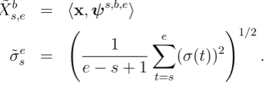
In our data, change points occur at arbitrary locations and we hope to be able to capture this feature by the use of a suitably flexible oscillatory basis that permits adaptive choice of change points in the basis vectors, allowing for a sparse repre-sentation of the piecewise-constant trend. Arguably the simplest such construction is furnished by the Unbalanced Haar wavelets. With _I(·) denoting the indicator function, the elements of a generic UH vector ψs,b,e are

ψs,b,e(t) =

1

b−s+ 1 − 1

e−s+ 1

1/2

I(s≤t ≤b)

−

1

e−b −

1

e−s+ 1

1/2

I(b+ 1 ≤t ≤e),

where s and e are, respectively, the start- and end-point of its support, and b is the location of a change point. ψs,b,e is constant and positive before the change point, constant and negative after the change point, and such that P

tψs,b,e(t) = 0

and P

t(ψ

s,b,e₍_t₎₎2 _{= 1. If constructed as follows, a set of (}_T ₋_{1) UH vectors plus}

(68)

basis vectorψb0,1 ₌_ψ1,b0,1,T_{; the change point} _b

0,1 needs to be chosen and we later

say how. Then, repeat this construction following the binary segmentation logic on the two parts of the domain determined by b0,1: provided that b0,1 ≥ 2, define

ψb1,1 ₌_ψ1,b1,1,b0,1_{, and provided that} _T ₋_b

0,1 ≥2, define ψb1,2 =ψb0,1+1,b1,2,T. The

recursion then continues in the same manner for as long as feasible, with each vector ψbj,k having at most two children vectors ψbj+1,2k−1 _and _ψbj+1,2k_{. Additionally, we}

define a vector ψb−1,0 _{with elements} _ψb−1,0₍_t_{) =} _T−1/2

I(1≤ t ≤ T). The indices j

and k are scale and location parameters, respectively. The larger the value of j, the finer the scale, as in the classical wavelet theory.

Example. We consider an example of a set of UH vectors for T = 6. The rows

of the matrixW defined below contain (from top to bottom) vectors ψb−1,0_,_ψb0,1_,

ψb1,2_, _ψb2,3_, _ψb2,4 _and