Orthogonal Polynomials of Compact Simple Lie Groups

(1)

Volume 2011, Article ID 969424,23pages doi:10.1155/2011/969424

Research Article

Orthogonal Polynomials of Compact Simple

Lie Groups

Maryna Nesterenko,

1

Jiˇr´ı Patera,

2

and Agnieszka Tereszkiewicz

3

1_{Department of Applied Research, Institute of Mathematics of NAS of Ukraine, 3 Tereshchenkivs’ka Street,}

Kyiv-4 01601, Ukraine

2_{Centre de Recherches Mathématiques, Université de Montréal, C.P.6128-Centre Ville, Montréal,}

QC H3C 3J7, Canada

3_{Institute of Mathematics, University of Bialystok, Akademicka 2, 15-267 Bialystok, Poland}

Correspondence should be addressed to Maryna Nesterenko,[email protected]

Received 28 December 2010; Revised 26 May 2011; Accepted 4 June 2011

Academic Editor: N. Govil

Copyrightq2011 Maryna Nesterenko et al. This is an open access article distributed under the Creative Commons Attribution License, which permits unrestricted use, distribution, and reproduction in any medium, provided the original work is properly cited.

Recursive algebraic construction of two infinite families of polynomials in n variables is proposed as a uniform method applicable to every semisimple Lie group of rank n. Its result recognizes Chebyshev polynomials of the first and second kind as the special case of the simple group of type A1. The obtained not Laurent-type polynomials are equivalent to the partial cases of the Macdonald

symmetric polynomials. Recurrence relations are shown for the Lie groups of types A1, A2, A3, C2,

C3, G2, and B3together with lowest polynomials.

1. Introduction

The majority of special functions and orthogonal polynomials introduced during the last dec-ade are associated with Lie groups or their generalizations. In particular, special functions of mathematical physics are in fact matrix elements of representations of Lie groups1and re-cent multivariate generalizations of classical hypergeometric orthogonal polynomials are based on root systems of simple Lie groups/algebras2–9. In this connection a number of el-egant results in theory of these polynomials, such as explicitdeterminantalcomputation of polynomials10–12and Pieri formulas13,14, were obtained, see also15–17and referen-ces therein.

(2)

building blocks in all multivariate polynomials associated with root systems. Unlike Gram-Schmidt type orthogonalization of the monomial basis with respect to Haar measure3,7,8 or determinantal construction of polynomials10–12we make profit from decomposition of products of Weyl group orbits and from basic properties of the characters of irreducible finite dimensional representations.

Our method is purely algebraic and we propose three diﬀerent ways to transform aC -or S-orbit function into a polynomial. The first one substitutes for each multivariable ex-ponential term in an orbit function a monomial of as many variables. In 1D this results in Chebyshev polynomials written as Laurent polynomials with symmetrically placed positive and negative powers of the variable; and in the case ofA2 our results coincide with those from18.

The second transformation, the “truly trigonometric” form, is based on the fact that, for many simple Lie algebrassee the list in3.3below, eachCandS-orbit function consists of pairs of exponential terms that add up to either cosine or sine. Hence such a function is a sum of trigonometric termsor a polynomial of one-dimensional Chebyshev polynomials. For the Chebyshev polynomials we obtain in this way their trigonometric form. Note from

3.3that this method does not apply to the groupsAnforn >1.

But this paper focuses on polynomials obtained by the third substitution of variables, mimicking Weyl’s method for the construction of finite-dimensional representations fromn

fundamental representations. Thus theCpolynomials havenvariables that are theC-orbit functions, one for each fundamental weightωj. This approach results in a simple recursive

construction that allows one to represent any orbit function/monomial symmetric function in non-Laurent polynomial form.

In addition to the general approach and associated tools we present a lot of explicit and practically useful data and discussions, namely, inAppendix Awe compare the classical Chebyshev polynomialsDickson polynomialsand orbit functions ofA1with their recursion relations. Suitably normalized, the Chebyshev polynomials of the first and second kind coincide with theCandSpolynomials. A table of the polynomials of each kind is presented. AppendicesB,C, andDcontain, respectively, the recursion relations for polynomials of the Lie algebrasA2,C2, andG2. InAppendix Erecursion relations forA3,B3, andC3polynomials of both kinds are listed together with useful tools for solving these recursion relations.

2. Preliminaries and Conventions

This section serves to fix notations and terminology, additional details can be found for ex-ample in19–26.

LetRn _{be the Euclidean space spanned by the simple roots of a simple Lie group}_G_.

The basis of the simple roots and the basis of fundamental weights are hereafter referred to as theα-basis andω-basis, respectively. Bases dual toα- andω-bases are denoted by ˇα- and

ˇ

ω-bases. In addition we use{e1, . . . , en}, the orthonormal basis ofRn. The root latticeQand

the weight latticePofGare formed by all integer linear combinations of theα-basis andω -basis, respectively. InP we define the cone of dominant weightsP and its subset of strictly dominant weightsP.

HereafterWWGis the Weyl group of size|Wλ|, andWλis the orbit containing the dominantpointλ ∈P ⊂Rn_{. The fundamental region}_F_G_⊂_Rn_{is the convex hull of the}

(3)

Definition 2.1. TheC-functionCλxis defined as

Cλx:

μ∈WλG

e2πiμ,x, x∈Rn, λ∈P. 2.1

Occasionally it is useful to scale upCλof nongenericλby the stabilizer ofλinW.

Definition 2.2. TheS-functionSλxis defined as

Sλx:

μ∈WλG

−1pμe2πiμ,x, x∈Rn, λ∈P, 2.2

wherepμis the number of elementary reflections necessary to obtainμfromλ.

In this paper, we always suppose thatλ, μ∈Pare given inω-basis andx∈Rn_{is given}

in ˇα-basis, hence the orbit functions have the following forms:

Cλx

μ∈Wλ

e2πinj1μjxj

μ∈Wλ

n

j1

e2πiμjxj_,

Sλx

μ∈Wλ

−1pμe2πinj1μjxj

μ∈Wλ

−1pμ

n

j1

e2πiμjxj_.

2.3

There is a fundamental relation between theC- andS-orbit functions for simple Lie groupGof any type and rank, called the Weyl character formula:

χλx

Sλρx

Sρx

μ

mλμCμx, x∈Rn, λ, μ∈P, ρ

n

k1

ωk. 2.4

The positive integermλ

μis the Kostka number27,28.

The rank of the underlying semisimple Lie group/algebra is the number of variables of the orbit functions.CandSfunctions are continuous and have continuous derivatives; they are, respectively, symmetric and antisymmetric with respect to then−1-dimensional bound-ary ofF23–25. Moreover, any pair of orbit functions from the same family is orthogonal on the corresponding fundamental region20, these families of functions are complete, and

Cλx- andSλx-orbit functions are eigenfunctions of then-dimensional Laplace operator.

3. Multivariate Orthogonal Polynomials Corresponding to

Orbit Functions

In this section we consider several transformations

T:Rn−→Cn; x1, . . . , xn−→X1, . . . , Xn, 3.1

(4)

It directly follows from the orthogonality of the orbit functions that such polynomials are orthogonal on the domainFwith the weight function det−1_D_X_/D_x_{, where}_F_{is the} image of the fundamental regionFunder the transformationT.

iThe first type of transformation is rather straightforward

Xj:e2πixj, xj∈R, j1,2, . . . , n. 3.2

Polynomial summands are productsn_j₁Xμj

j , where μj ∈ Zare components of the

orbit points relative to a suitable basis. Under this transformation orbit function,Cλxand

Sλx, given by2.3, become Laurent polynomials innvariablesXj, wherej {1,2, . . . , n}.

The exponential substitution polynomials are complex-valued in general, admit neg-ative powers, and have all their coeﬃcients equal to one inCpolynomials, and 1 or−1 inS

polynomials.

iiTheW-orbits of the Lie groups

A1, Bn n≥3, Cn n≥2, D2n n≥2, E7, E8, F4, G2 3.3

have an additional property±μ ∈ WλLfor allμ ∈WλL, then the pair of corresponding

terms of the function ofWλLcan be combined so thatCλxandSλxbecome linear

com-binations of cosines and sines:

e2πiμ,xe−2πiμ,x2 cos2πμ, x ∈Cλx,

e2πiμ,x−e−2πiμ,x2isin2πμ, x ∈Sλx,

3.4

that admits a truly trigonometric substitution of variables. Note that in the case ofA1, this is precisely the trigonometric substitution made for Chebyshev polynomials of the first and second kind.

Remark 3.1. Chebyshev polynomials of one variable play crucial role for the orbit functions of the above-mentioned Lie groups as far as they allow us to calculate the polynomial coeffi-cients explicitly.

Really, as far as we suppose that λ are given in ω-basis and x is given in ˇα-basis, then, using common trigonometric identities, cosines and sines can be expressed through the cosines and sines of 2πkxi,k ∈N,i 1, . . . , n. What immediately represents our orbit

func-tions as polynomials of Chebyshev polynomials of the firstTkxiand second Ukxikind

with well-known formulas for coeﬃcients.

iiiThe third transformation, which we propose here, works uniformly for simple Lie algebras of all types. We chooseCfunctions of thenfundamental weights as thennew variables:

Xj :Xjx:Cωjx, j 1,2, . . . , n, x∈R

(5)

completed by one more variable, the lowestSfunction,

S :Sρx, x∈Rn, ρ 1,1, . . . ,1

n

m1

ωm. 3.6

The recursive construction ofC-polynomials begins by multiplying the variablesXj and C

-functions and decomposing their products into sums ofC-polynomials. A judicious choice of the sequence of products allows one to find ever higher degreeC-polynomials.

First, generic recursion relations are found as the decomposition of products

XjCa1,a2,...,anwith “suﬃciently large”a1, a2, . . . , ani.e., allCfunctions in the decomposition

should correspond to generic points. Then the rest of necessary recursions“additional”are constructed. An eﬃcient way to find the decompositions is to work with products of Weyl group orbits, rather than with orbit functions. Their decomposition has been studied, and many examples have been described in29. Note that these recursion relations are always linear and the corresponding matrix is triangular. The procedure is exemplified in Appendi-cesA–Efor Simple Lie groups of ranks 1, 2, and 3.

Results of the recursive procedures can be summarized as followssee30for the proof.

Proposition 3.2. Any irreducibleC-function and any characterχλof a simple Lie groupGcan be

rep-resented as a polynomial ofC-functions of the fundamental weightsω1, . . . , ωn, that is, a polynomial

in the variablesX1, X2, . . . , Xn.

The recursive construction of S-polynomials starts by multiplying the variablesS and

Xj and decomposing their products into sums ofS polynomials. However, the higher the

rank of the underlying Lie algebra, the recursive procedure forSpolynomials becomes more laborious, what caused by the presence of negative terms inSpolynomials. Fortunately, there is an alternative to the recursive procedure. Once theCpolynomials have been calculated, they can be used in Weyl character formula for findingSpolynomials as sums ofC polyno-mials multiplied by the variableS. In practice, polynomialsSλ/S should be used instead of

Sλ.

Remark 3.3. There are two easy and practical checks on recursion relations applicable to all simple Lie algebras. The first one is the equality of numbers of exponential terms inS- orC -functions on both sides of a recursion relationthe numbers of exponential terms are calcu-lated using the sizes of Weyl group orbits. The second check is the equality of congruence numbers.

Remark 3.4. Polynomial forms ofCandSfunctions introduced in this section are partial cases of the Macdonald symmetric polynomials.

All C- andS-orthogonal polynomialsand, therefore, the Macdonald polynomials inherit from orbit functions important discretization properties. A uniform discretization of these polynomials follows from their invariance with respect to the aﬃne Weyl group ofG

and from the well-established discretization of the fundamental regionFG 20. One more advantage is the cubature formula introduced in31.

(6)

both generic and additional recursions or, instead of cumbersome additional recursions, we present all their solutions in form of lowest polynomials. The skipped explicit formulas are available in30,32.

The content of AppendicesA–Eis also motivated by the fact that calculation of addi-tional recurrences is not suitable for complete computer automatization. However, as soon as additional recurrencesor their solutionswere obtained, all other calculations concerning polynomials and their applications become very algorithmic and can easily be done by com-puter algebra packages for Lie theory.

4. Conclusion

There is an alternative way to our construction of the polynomials in all but in theAncases.

The crucial substitution3.5can be replaced by

Xk:χωkx, k1,2, . . . , n. 4.1

In4.1the variables are characters of irreducible representations with highest weights given as the fundamental weights, while in3.5the variables areCfunctions of the fundamental weights. Only forAnthe two coincide,Cωkx χωkxfor allk1, . . . , nand for allx∈Rn.

Already for the rank two cases other than A2 there is a diﬀerence. Indeed, 4.1reads as follows:

C2:X1χω1x Cω1x, X2χω2x Cω2x 2,

G2:X1χω1x Cω1x Cω2x 2, X2χω2x Cω2x 1.

4.2

Since products of characters decompose into their sum, the recursive construction can pro-ceed, but the polynomials will be diﬀerent.

For simplicity of formulation, we insisted throughout this paper that the underlying Lie group be simple. The extension to compact semisimple Lie groups and their Lie algebras is straightforward. Thus, orbit functions are products of orbit functions of simple constituents, and diﬀerent types of orbit functions can be mixed.

Polynomials formed from other orbit functionsE-,E−-,E-,S-,S−-,C-,C− -func-tionsby the same substitution of variables should be equally interesting oncen > 1. These functions have been studied in20,25,26,33.

Appendices

A. Orbit Functions of

A

1

, Their Polynomial Forms,

and Chebyshev Polynomials

(7)

TheC-polynomials generated by our approach are naturally normalized in a diﬀerent way than the classical polynomialsthey coincide with the form of Dickson polynomials.

The orbit functions ofA1are of two types:

Cmx e2πimxe−2πimx2 cos2πmx, x∈R, m∈Z>0,

Smx e2πimx−e−2πimx2isin2πmx, x∈R, m∈Z>0.

A.1

We introduce new variablesXandSas follows:

X :C1x e2πixe−2πix2 cos2πx,

S:S1x e2πix−e−2πix2isin2πx.

A.2

Polynomials can now be constructed recursively in the degrees ofXandSby calculating the decompositions of products of appropriate orbit functions. “Generic” recursion relations are those where one of the first degree polynomials,XorS, multiplies the generic polynomialCm

orSm, that is,m≥1. Omitting the dependence onxfrom the symbols, we have the generic

recursion relations

XCmCm1Cm−1, SCmSm1−Sm−1,

XSmSm1Sm−1, SSmCm1−Cm−1, m1. A.3

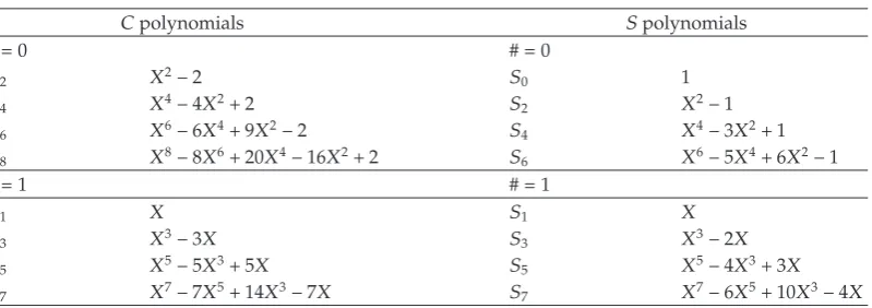
When solving recursion relations forCpolynomials, we need to start from the lowest ones; several results are inTable 1. Hence we conclude thatCm2Tm, form0,1, . . ..

The characterχmxof an irreducible representation ofA1of dimensionm1 is known explicitly for allm0. There are two ways to write the character: as the ratio ofS-functions, and as the sum ofC-functions. Explicitly, that is

SmX χmx Sm1x

Sx Cmx Cm−2x · · · ⎧ ⎨ ⎩

C2x C0 ifmeven,

C3x C1x ifmodd.

A.4

Note thatA.4is the Chebyshev polynomial of the second kindUmx.

Remark A.1. The main argument in favor of our normalization of Chebyshev polynomials is that polynomialsCm fromTable 1are Dickson polynomialsit is well known that they are

equivalent to Chebyshev polynomials over the complex numbers. It is easy to provesee e.g., 40 that Weyl group ofAn is equivalent to Sn1, therefore it is natural to consider multivariateC-polynomials ofAnasn-dimensional generalizations of Dickson polynomials as permutation polynomials. Also our form of Dickson-Chebyshev polynomials makes them the lowest special case of 2.4 without additional adjustments and it appears more “natural” because, for example, the equalityC2

(8)

[image:8.600.105.505.111.252.2]

Table 1: The irreducibleCandSpolynomials ofA1of degrees up to 8.

Cpolynomials Spolynomials

#0 #0

C2 X2₋₂ _S0 ₁

C4 X4₋₄_X2₂ _S2 _X2₋₁

C6 X6₋₆_X4₉_X2₋₂ _S4 _X4₋₃_X2₁

C8 X8₋₈_X6₂₀_X4₋₁₆_X2₂ _S6 _X6₋₅_X4₆_X2₋₁

#1 #1

C1 X S1 X

C3 X3₋₃_X _S3 _X3₋₂_X

C5 X5₋₅_X3₅_X _S5 _X5₋₄_X3₃_X

C7 X7₋₇_X5₁₄_X3₋₇_X _S7 _X7₋₆_X5₁₀_X3₋₄_X

B. Recursion Relations for

A

2

Orbit Functions and Polynomials

The variables of the A2 polynomials are the C functions of the lowest dominant weights

ω1 1,0andω2 0,1:

X1:C1,0x1, x2, X2:C0,1x1, x2, S:S1,1x1, x2. B.1

We omit writingx1, x2at the symbols of orbit functions for simplicity of notations.

In addition to the obvious polynomialsX1,X2,X2₁,X1X2, andX₂2, we recursively find the rest of theA2-polynomials. The degree of the polynomialCa,bequalsab. The degree

ofSa,bis alsoabprovidedab /0, otherwise theS-polynomials are zero.

Due to theA2 outer automorphism, polynomialsCa,b and Cb,a are related by the interchange of variablesX1↔X2i.e.Ca,bX1, X2 Cb,aX2, X1.

In general, each term in an irreducible polynomial, equivalently each weight of an orbit, must belong to the same congruence class specified by the congruence number #. For

A2-weighta, b, we have

#a, b a2bmod 3. B.2

Hence, irreducible orbit functions have a well-defined value of #. ForA2-orbit functions, we have #Ca,b #Sa,b a2bmod 3. Consequently, there are three classes of polyno-mials corresponding to # 0,1,2. During multiplication, the congruence numbers add up mod 3. A product of irreducible orbits decomposes into the sum of orbits belonging to the same congruence class. The sizes of the irreducible orbits ofWA2 are found in30. The dimensionda,bof the representation ofA2with the highest weighta, bis given byda,b

1/2a1b1ab2.

B.1. Recursion Relations for

C

-Function Polynomials of

A

2

(9)

X1Ca,bCa1,bCa−1,b1Ca,b−1, a, b2,

X2Ca,bCa,b1Ca1,b−1Ca−1,b, a, b2.

B.3

Before generic recursion relations can be used, the special recursion relations for particular valuesa, b∈ {0,1}need to be solved recursively starting from the lowest ones:

X12C2,02X2, X22C0,22X1, X1X2C1,13,

X1C1,1C2,12C0,22X1, X2C1,1C1,22C2,02X2,

B.4

fora2:

X1Ca,1Ca1,1Ca−1,22Ca,0, X2Ca,1Ca,22Ca1,0Ca−1,1,

X1Ca,0 Ca1,0Ca−1,1, X2Ca,0Ca,1Ca−1,0,

B.5

forb2:

X1C1,b C2,b2C0,b1C1,b−1, X2C1,bC1,b1C2,b−12C0,b,

X1C0,b C1,bC0,b−1, X2C0,bC0,b1C1,b−1.

B.6

Using the symmetry of orbit functions with respect to the permutation of the components of dominant weights, we obtain analogous polynomialsCa,0andCa,1for alla∈N. Then the 4-term special recursion relations are solved yieldingC2,bandCa,2 for alla, b ∈ N. After that, the generic recursion relations should be used.

B.2. The Character of

A

2

In theA2case the general formula2.4is specialized

Sa,bX1, X2 χa,bx, y Sa1,b1

x, y

S1,1x, y Ca,b

x, y

λ

mλCλ

x, y. B.7

The summation extends over the dominant weights that have positive multiplicitiesmλ in

the case ofχa,b. The coeﬃcientsdominant weight multiplicitiesare tabulated in27for the 50 firstχa,bin each congruence class ofA2. The first few characters for the congruence class #0 are

χ0,0C0,01,

χ1,1C1,12C0,0,

χ3,0C3,0C1,1C0,0,

(10)

χ2,2C2,2C0,3C3,02C1,13C0,0,

χ1,4C1,4C2,22C0,3C3,02C1,12C0,0,

χ3,3C3,3C4,1C1,42C2,22C0,32C3,03C1,14C0,0,

χ6,0C6,0C4,1C2,2C0,3C3,0C1,1C0,0.

B.8

The equalities must satisfy two relatively simple conditions:ithe dominant weights on both sides must have the same congruence numberB.2, andiithe number of exponential terms in a character χa,b is known to be the dimension of the irreducible representationa, b. Therefore, the sizes of the orbit functions on the right side have to add up to the dimension.

For #1:

χ1,0 C1,0,

χ0,2 C0,2C1,0,

χ2,1 C2,1C0,22C1,0,

χ1,3 C1,3C2,12C0,22C1,0,

χ4,0 C4,0C2,1C0,2C1,0,

χ0,5 C0,5C1,3C2,1C0,2C1,0.

B.9

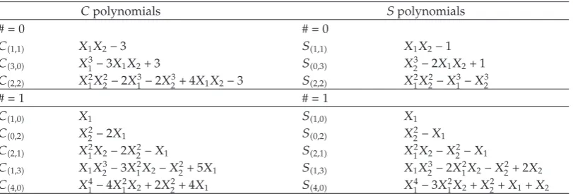
For # 2, it suﬃces to interchange the component of all dominant weights in the equalities for #1. Thus no independent calculation is needed, seeTable 2for the solution.

C. Recursion Relations for

C

2

Orbit Functions

There are two congruence classes ofC2 orbit functions/polynomials. ForC2 weighta, b

dominant or not, we have

#a, b amod 2. C.1

The dimensionda,bof an irreducible representation ofC2 with the highest weighta, bis given by

da,b

1

6a1b12ab3ab2. C.2

In multiplying the polynomials, congruence numbers add up mod 2. Character in the case ofC2is given by2.4, where theCandSfunctions are those ofC2, as are the coeﬃcients

(11)

[image:11.600.100.506.124.263.2]

Table 2: The irreducibleC- andS-polynomials ofA2of degree up to 4. From any polynomialCa,borSa,b we obtainCb,aorSb,a, respectively, by interchangingX1andX2.

#0 #0

C1,1 X1X2−3 S1,1 X1X2−1

C3,0 X13−3X1X23 S0,3 X23−2X1X21

C2,2 X12X22−2X13−2X234X1X2−3 S2,2 X12X22−X31−X23

#1 #1

C1,0 X1 S1,0 X1

C0,2 X22−2X1 S0,2 X22−X1

C2,1 X2

1X2−2X22−X1 S2,1 X12X2−X22−X1

C1,3 X1X32−3X21X2−X225X1 S1,3 X1X23−2X21X2−X222X2

C4,0 X14−4X12X22X224X1 S4,0 X14−3X12X2X22X1X2

We denote the variables of theC2-polynomials by

X1:C1,0x, y, X2:C0,1x, y, and S:S1,1x, y, Sa,bX1, X2 χa,bx, y

C.3

often omitting x, y from the symbols. The variable S cannot be built out of X1 and X2. Although the variables are denoted by the same symbols as in the case ofA2 and alsoG2 below, they are very diﬀerent. ThusX1andX2contain 4 exponential terms andScontains 8 terms. The congruence number # ofX1andSis 1, while that ofX2is 0.

C.1. Recursion Relations for

C

Functions of

C

2

The two generic recursion relations forC-functions ofC2are

X1Ca,bCa1,bCa−1,b1Ca1,b−1Ca−1,b, a, b2,

X2Ca,bCa,b1Ca2,b−1Ca−2,b1Ca,b−1, a3, b2.

C.4

The special recursion relations forC-functions involving low values ofaandbhave to be solved first starting from the lowest ones:

X1Ca,1Ca1,1Ca−1,22Ca1,0Ca−1,1, a2,

X1Ca,0Ca1,0Ca−1,1Ca−1,0, a2,

X1C1,bC2,b2C0,b1C2,b−12C0,b, b2,

X1C0,bC1,bC1,b−1, b2,

X1C1,1C2,12C0,22C2,02X2,

(12)

X2Ca,1Ca,22Ca2,0Ca−2,22Ca,0, a3,

X2Ca,0Ca,1Ca−2,1, a3,

X2C2,bC2,b1C4,b−12C0,b1C2,b−1, b2,

X2C1,bC1,b1C3,b−1C1,b−1C1,b, b2,

X2C0,bC0,b1C2,b−1C0,b−1, b2,

X2C2,1C2,22C4,0C0,42C0,22C2,0,

X2C1,1C1,22C3,0C1,12X1,

X2C2,0C2,12X2; X22C0,22C2,04.

C.5

The 3- and 4-term recursion relations are solved independently, giving usC0,b,Ca,0,

C1,b, andCa,1for allaandb, for example, seeTable 3.

C.2. Recursion Relations for

S

Functions of

C

2

The generic relations for S functions are readily obtained from those of C functions by replacingCbyS, and by making appropriate sign changes.

AllCfunctions ofC2are real valued. Here are a few examples ofC2characters:

#0:

χ0,0C0,01,

χ0,11C0,1 1X2,

χ2,02X2C2,0,

χ0,22X2C2,0C0,2,

χ2,133X22C2,0C0,2C2,1,

χ0,322X2C2,0C0,2C2,1C0,3,

χ4,032X22C2,0C0,2C2,1C4,0,

χ2,254X24C2,03C0,22C2,1C0,3C4,0C2,2,

#1:

χ1,0C1,0X1,

(13)

χ3,02X1C1,1C3,0,

χ1,23X12C1,1C3,0C1,2,

χ3,14X13C1,12C3,0C1,2C3,1,

χ1,34X13C1,12C3,02C1,2C3,1C1,3.

C.6

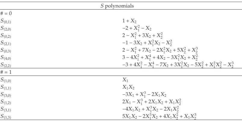
Using these characters andTable 3, we can calculate all irreducibleSpolynomials of degree up to four with respect to the variablesX1andX2, seeTable 4. Note thatχ0,4yields the polynomial of order five.

D. Recursion Relations for

G

2

Orbit Functions

AllG2weights fall into the same congruence class #0. Thus there are no congruence classes to distinguish inG2. The variables are the orbit functions of the two fundamental weights:

X1:C1,0x, y, X2:C0,1x, y, SS1,1x, y, Sa,bX1, X2 χa,bx, y.

D.1

D.1. Recursion Relations for

C

Functions of

G

2

There are two generic recursion relations forCpolynomials ofG2, each containing one prod-uct term and sixCpolynomials.

Fora3, b4:

X1Ca,bCa1,bCa−1,b3Ca2,b−3Ca−2,b3Ca1,b−3Ca−1,b.

Fora2, b3:

X2Ca,bCa,b1Ca1,b−1Ca−1,b2Ca1,b−2Ca−1,b1Ca,b−1.

D.2

Specializing the first of the generic relations to eithera∈ {0,1,2}orb∈ {0,1,2,3}, we have

X1C2,bC3,bC1,b3C4,b−32C0,b3C3,b−3C1,b,

X1C1,bC2,b2C0,b3C3,b−3C2,b−3C1,b2C0,b,

X1C0,bC1,bC2,b−3C1,b−3,

X1Ca,3Ca1,3Ca−1,62Ca2,0Ca−2,62Ca1,0Ca−1,3,

X1Ca,2Ca1,2Ca−1,5Ca1,1Ca−2,5Ca,1Ca−1,2,

(14)

X1Ca,0Ca1,0Ca−1,3Ca−2,3Ca−1,0,

X1C2,3C3,3C1,62C4,02C0,62C3,0C1,3,

X1C2,2C3,2C1,5C0,5C1,2C2,1C3,1,

X1C2,1C3,1C1,42C0,4C1,1C2,2C1,2,

X1C2,0C3,0C1,32C0,3X1,

X1C1,3C2,32C0,62C3,02C2,0C1,32C0,3,

X1C1,2C2,22C0,5C1,22C0,2C2,1C1,1,

X1C1,1C2,12C0,4C1,22C0,2C1,12X2,

X1C0,3C1,32C2,02X1,

X1C0,2C1,2C1,12X2,

X1X1 C2,02C0,32X16,

X1X2 C1,12C0,22X2.

D.3

Specializing the second of the generic relations to eithera∈ {0,1}orb∈ {0,1,2}, we have

X2C1,bC1,b1C2,b−12C0,b2C2,b−22C0,b1C1,b−1,

X2C0,bC0,b1C1,b−1C1,b−2C0,b−1,

X2Ca,1 Ca,22Ca1,0Ca−1,3Ca−1,22Ca,0Ca,1,

X2Ca,0 Ca,1Ca−1,2Ca−1,1,

X2C1,2C1,3C2,12C0,42C0,3C1,12C2,0,

X2C1,1C1,22C2,02C0,32C0,2C1,12X1,

X2C0,2C0,3C1,12X1X2,

X2X2C0,22X12X26.

D.4

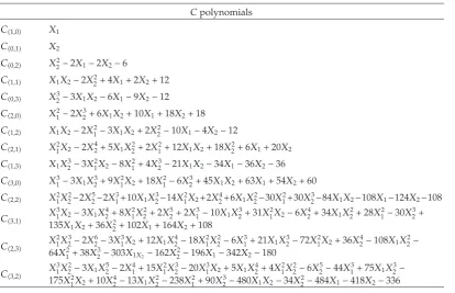
Remark D.1. It can be seen fromTable 5 that order ofCa,b polynomial sometimes exceeds

(15)

[image:15.600.102.504.110.325.2]

Table 3: The irreducibleCpolynomials ofC2of degree up to 4.

Cpolynomials #0

C0,1 X2

C2,0 X21−2X2−4

C2,1 X2

1X2−2X22−6X2

C4,0 4−4X21X148X2−4X12X22X22

C0,2 4−2X214X2X22

C0,3 9X2−3X12X26X

2

2X

3 2

C2,2 −810X12−2X14−20X28X21X2−12X22X12X22−2X23

C0,4 4−8X122X4116X2−8X12X220X22−4X12X228X23X42

#1

C1,0 X1

C1,1 X1X2−2X1

C3,0 X31−3X1X2−3X1

C3,1 2X1−4X1X2X13X2−3X1X22

C1,2 6X1−2X133X1X2X1X22

C1,3 −6X12X316X1X2−3X

3

1X25X1X

2

2X1X

3 2

Table 4: The irreducibleSpolynomials ofC2of degree up to 4.

Spolynomials #0

S0,1 1X2

S2,0 −2X12−X2

S0,2 2−X123X2X

2 2

S2,1 −1−3X2X12X2−X22

S0,3 2−X127X2−2X12X25X22X23

S4,0 3−4X12X

4

14X2−3X

2

1X2X

2 2

S2,2 −34X21−X41−7X23X12X2−5X22X12X22−X

3 2

#1

S1,0 X1

S1,1 X1X2

S3,0 −3X1X31−2X1X2

S1,2 2X1−X312X1X2X1X

2 2

S3,1 −4X1X2X13X2−2X1X22

S1,3 5X1X2−2X31X24X1X22X1X32

D.2. Recursion Relations for

S

Functions of

G

2

Generic recursion relations forSpolynomials diﬀer very little from those forCpolynomials.

Fora3, b4:

[image:15.600.99.502.367.569.2]

(16)

Fora2, b3:

X2Sa,bSa,b1Sa1,b−1Sa−1,b2Sa1,b−2Sa−1,b1Sa,b−1.

D.5

TheS polynomials need not be calculated independently. They can be read oﬀthe tables27as the characters ofG2representations, seeTable 6.

Here are allG2-charactersχa,bwithab3:

χ1,0 1C1,01X1,

χ0,1 2C1,0C0,1 2X1X2,

χ2,0 32X1X2C2,0,

χ1,1 44X12X22C2,0C1,1,

χ3,0 54X13X22C2,0C3,0,

χ0,2 53X13X22C2,0C1,1C3,0C0,2,

χ2,1 98X16X25C2,03C1,12C3,0C0,2C2,1,

χ1,2 1010X17X27C2,05C1,13C3,03C3,02C0,22C2,1C4,0C1,2,

χ0,3 97X17X25C2,04C1,14C3,03C0,22C1,1C4,0C1,2,

C3,1C0,3.

D.6

E. Recursion Relations for Lie Algebras of Rank 3

E.1. Recursion Relations for

C

-Functions of

A

3

There are 4 congruence classes ofA3defined by

#a, b, c a2b3cmod 4. E.1

The variables of theA3polynomials are chosen to be

X1:C1,0,0x1, x2, x3, X2:C0,1,0x1, x2, x3,

X3:C0,0,1x1, x2, x3andSa,b,cX1, X2, X3 χa,b,cx, y, z.

(17)

[image:17.600.98.513.112.379.2]

Table 5: The irreducibleCa,bpolynomials ofG2.

Cpolynomials

C1,0 X1

C0,1 X2

C0,2 X22−2X1−2X2−6

C1,1 X1X2−2X224X12X212

C0,3 X32−3X1X2−6X1−9X2−12

C2,0 X2

1−2X

3

26X1X210X118X218

C1,2 X1X2−2X21−3X1X22X

2

2−10X1−4X2−12

C2,1 X21X2−2X

4

25X1X222X

2

112X1X218X

2

26X120X2

C1,3 X1X23−3X

2

1X2−8X

2

14X

3

2−21X1X2−34X1−36X2−36

C3,0 X31−3X1X

3

29X

2

1X218X

2

1−6X

3

245X1X263X154X260

C2,2 X21X

2

2−2X

5

2−2X

3

110X1X

3

2−14X

2

1X22X

4

26X1X

2

2−30X

2

130X

3

2−84X1X2−108X1−124X2−108

C3,1 X

3

1X2−3X1X428X21X222X522X31−10X1X2331X21X2−6X2434X1X2228X21−30X32

135X1X236X2

2102X1164X2108

C2,3 X

2

1X

3

2−2X

6

2−3X

3

1X212X1X24−18X12X22−6X

3

121X1X

3

2−72X21X236X42−108X1X22−

64X2

138X32−303X1X2−162X

2

2−196X1−342X2−180

C3,2 X

3

1X

2

2−3X1X

5

2−2X

4

115X

2

1X

3

2−20X

3

1X25X1X

4

24X

2

1X

2

2−6X

5

2−44X

3

175X1X

3

2−

175X2

1X210X24−13X1X22−238X2190X23−480X1X2−34X22−484X1−418X2−336

Table 6: The irreducibleSa,bpolynomials ofG2withab5.

Spolynomials

S0,1 X21

S1,0 X1X22

S0,2 X22−X1−3

S1,1 X1X22X12X24

S2,0 X21−X234X1X27X110X211

S1,2 X1X22−X

2

1X

2

2−4X1−3

S2,1 X21X2−X243X1X222X12−X

3

210X1X29X229X119X210

S2,2 X21X22−X25−X314X1X23−3X12X26X1X22−9X1212X23−18X1X29X22−27X1−27X2−27

For C functions the generic recursion relations are the following ones, where we assumea, b, c2:

X1Ca,b,cCa1,b,cCa−1,b1,cCa,b−1,c1Ca,b,c−1,

X2Ca,b,cCa,b1,cCa1,b−1,c1Ca−1,b,c1Ca1,b,c−1Ca−1,b1,c−1Ca,b−1,c,

X3Ca,b,cCa,b,c1Ca,b1,c−1Ca1,b−1,cCa−1,b,c.

E.3

Note that the first and the third relations are easily obtained from each other by interchanging the first and third component of all dominant weights. Thus X1 ↔ X3 and a, b, c ↔

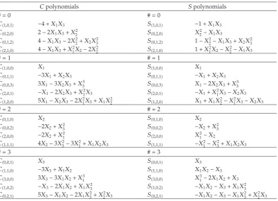
[image:17.600.109.505.409.532.2]

(18)

[image:18.600.102.505.112.402.2]

Table 7: The irreducibleCpolynomials andSpolynomials ofA3.

#0 #0

C1,0,1 −4X1X3 S1,0,1 −1X1X3

C0,2,0 2−2X1X3X22 S0,2,0 X22−X1X3

C0,1,2 4−X1X3−2X2

2X2X23 S0,1,2 1−X22−X1X3X2X32

C2,1,0 4−X1X3X12X2−2X22 S2,1,0 1X21X2−X22−X1X3

#1 #1

C1,0,0 X1 S1,0,0 X1

C0,1,1 −3X1X2X3 S0,1,1 −X1X2X3

C0,0,3 3X1−3X2X3X33 S0,0,3 X1−2X2X3X33

C2,0,1 −X1−2X2X3X12X3 S2,0,1 −X1X21X3−X2X3

C1,2,0 5X1−X2X3−2X12X3X1X22 S1,2,0 X1X1X22−X21X3−X2X3

#2 #2

C0,1,0 X2 S0,1,0 X2

C0,0,2 −2X2X23 S0,0,2 −X2X23

C2,0,0 −2X2X21 S2,0,0 X

2

1−X2

C1,1,1 4X2−3X23−3X21X1X2X3 S1,1,1 −X21−X32X1X2X3

#3 #3

C0,0,1 X3 S0,0,1 X3

C1,1,0 −3X3X1X2 S1,1,0 X1X2−X3

C3,0,0 3X3−3X1X2X13 S3,0,0 X31−2X1X2X3

C1,0,2 −X3−2X1X2X1X23 S1,0,2 −X1X2−X3X1X

2 3

C0,2,1 5X3−X1X2−2X1X32X22X3 S0,2,1 −X1X2−X3−X1X32X22X3

The special recursion relations are obtained from the same products, where some of the componentsa,b,cof the generic dominant weight take special values 1 and 0. The explicit form of these relations is available in30and here we skip them in order to save the space, instead of this we adduce all their solutions of form ofTable 7.

E.2.

S

Polynomials of

A

3

Generic recursion relations are decompositions of the following products, where we assume

thata, b, c >1:

X1Sa,b,cSa1,b,cSa−1,b1,cSa,b−1,c1Sa,b,c−1,

X2Sa,b,cSa,b1,cSa1,b−1,c1Sa−1,b,c1Sa1,b,c−1Sa−1,b1,c−1Sa,b−1,c,

X3Sa,b,cSa,b,c1Sa,b1,c−1Sa1,b−1,cSa−1,b,c.

E.4

To calculateSpolynomials explicitlyseeTable 7we use theA3characters. The lowest ones from the congruence classes #0, #1, #2 and #3 are listed below:

#0:

χ0,0,0 C0,0,01,

(19)

χ0,2,0 2C1,0,1C0,2,0,

χ0,1,2 32C1,0,1C0,2,0C0,1,2,

χ2,1,0 32C1,0,1C0,2,0C2,1,0,

#1:

χ1,0,0 C1,0,0X1,

χ0,1,1 2X1C0,1,1,

χ2,0,1 3X1C0,1,1C2,0,1,

χ0,0,3 X1C0,1,1C0,0,3,

χ1,2,0 3X12C0,1,1C2,0,1C1,2,0,

#2:

χ0,1,0 C0,1,0X2,

χ0,0,2 X2C0,0,2,

χ2,0,0 X2C2,0,0,

χ1,1,1 4X22C0,0,22C2,0,0C1,1,1,

#3:

χ0,0,1 C0,0,1X3,

χ1,1,0 2X3C1,1,0,

χ1,0,2 3X3C1,1,0C1,0,2,

χ3,0,0 X3C1,1,0C3,0,0,

χ0,2,1 3X32C1,1,0C1,0,2C0,2,1.

E.3. Recursion Relations for

C

and

S

Polynomials of

B

3

and

C

3

The two cases diﬀer in many important respects in spite of the isomorphism of their Weyl groups.

We write the generic relations for the Cpolynomials of the Lie algebras B3 and C3

resp., of the simple Lie groupO7andSp6. The generic relations for theS-polynomials are obtained by replacing theCsymbol byS.

The variables are denoted by the same symbolsX1,X2,X3for all algebras of rank 3, namely,Xj :Cωj,j 1,2,3. There are two congruence classes ofa1, a2, a3for either of the

two algebras. We have

(20)

[image:20.600.106.507.113.366.2]

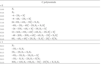
Table 8:Cpolynomials ofB3split into two congruence classes #0 and #1.

Cpolynomials #0

C1,0,0 X1

C0,1,0 X2

C2,0,0 −6−2X2X21

C0,0,2 −8−4X1−2X2X32

C1,1,0 248X16X2−3X32X1X2

C1,0,2 −8X1−2X2−4X12−2X1X2X1X

2 3

C3,0,0 −24−15X1−6X2X32−3X1X2X31

C0,2,0 1216X18X24X214X1X2−2X1X32X22

C0,1,2 −48−20X1−20X26X32−6X1X2−2X22X2X32

C2,1,0 8X1−6X24X122X1X2−X1X32−2X22X12X2

#1

C0,0,1 X3

C1,0,1 −3X3X1X3

C0,1,1 3X3−2X1X3X2X3

C0,0,3 −9X3−3X1X3−3X2X3X33

C2,0,1 −3X3−X1X3−2X2X3X21X3

C1,1,1 30X312X1X38X2X3−3X33−2X12X3X1X2X3

ForB3, we have the generic recursion relations

X1Ca,b,c Ca1,b,cCa−1,b1,cCa,b−1,c2Ca,b1,c−2Ca1,b−1,c

Ca−1,b,c, fora, b2, c3,

X2Ca,b,c Ca,b1,cCa1,b−1,c2Ca−1,b,c2Ca1,b1,c−2Ca−1,b2,c−2

Ca2,b−1,cCa1,b−2,c2Ca−2,b1,cCa−1,b−1,c2Ca1,b,c−2

Ca−1,b1,c−2Ca,b−1,c, a2, b, c3,

X3Ca,b,c Ca,b,c1Ca,b1,c−1Ca1,b−1,c1Ca−1,b,c1−Ca1,b,c−1

Ca−1,b1,c−1Ca,b−1,c1Ca,b,c−1, a, b, c2.

E.6

ForC3, we have the generic recursion relations

X1Ca,b,cCa1,b,cCa−1,b1,cCa,b−1,c1Ca,b1,c−1

Ca1,b−1,cCa−1,b,c, a, b, c2,

X2Ca,b,cCa,b1,cCa1,b−1,cCa−1,b,c1Ca1,b1,c−1Ca−1,b2,c−1

Ca2,b−1,cCa1,b−2,c1Ca−2,b1,cCa1,b,c−1Ca−1,b−1,c1

(21)

[image:21.600.150.452.112.387.2]

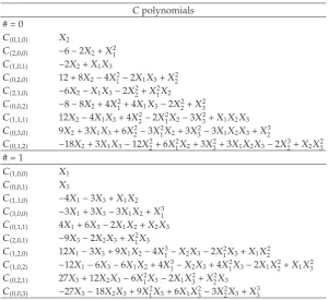
Table 9:Cpolynomials ofC3split into two congruence classes #0 and #1.

Cpolynomials #0

C0,1,0 X2

C2,0,0 −6−2X2X21

C1,0,1 −2X2X1X3

C0,2,0 128X2−4X21−2X1X3X22

C2,1,0 −6X2−X1X3−2X22X12X2

C0,0,2 −8−8X24X124X1X3−2X

2

2X

2 3

C1,1,1 12X2−4X1X34X22−2X21X2−3X32X1X2X3

C0,3,0 9X23X1X36X22−3X12X23X23−3X1X2X3X32

C0,1,2 −18X23X1X3−12X226X

2

1X23X

2

33X1X2X3−2X

3

2X2X

2 3

#1

C1,0,0 X1

C0,0,1 X3

C1,1,0 −4X1−3X3X1X2

C3,0,0 −3X13X3−3X1X2X13

C0,1,1 4X16X3−2X1X2X2X3

C2,0,1 −9X3−2X2X3X12X3

C1,2,0 12X1−3X39X1X2−4X13−X2X3−2X21X3X1X22

C1,0,2 −12X1−6X3−6X1X24X13−X2X34X

2

1X3−2X1X

2

2X1X

2 3

C0,2,1 27X312X2X3−6X12X3−2X1X32X22X3

C0,0,3 −27X3−18X2X39X12X36X1X23−3X22X3X33

X3Ca,b,cCa,b,c1Ca,b2,c−1Ca2,b−2,c1Ca−2,b,c1Ca2,b,c−1

Ca−2,b2,c−1Ca,b−2,c1Ca,b,c−1, a, b3, c2.

E.7

Additional recursion relations for both cases are available in explicit form in32and here we present only their solutions in form of Tables8and9.

Acknowledgments

This work supported in part by the Natural Sciences and Engineering Research Council of Canada, MITACS, and by the MIND Research Institute. M. Nesterenko and A. Tereszkiewicz are grateful for the hospitality extended to her at the Centre de Recherches Mathématiques, Université de Montréal, where a part of the work was carried out.

References

1 N. J. Vilenkin and A. U. Klimyk, Representation of Lie Groups and Special Functions: Recent Advances, vol. 316, Kluwer Academic Publishers, Dordrecht, The Netherlands, 1995.

2 C. F. Dunkl and Y. Xu, Orthogonal Polynomials of Several Variables, Cambridge University Press, New York, NY, USA, 2008.

(22)

4 T. H. Koornwinder, “Askey-Wilson polynomials for root systems of type BC,” in Hypergeometric Func-tions on Domains of Positivity, Jack Polynomials, and ApplicaFunc-tions (Tampa, FL, 1991), vol. 138 of Contempo-rary Mathematics, pp. 189–204, American Mathematical Society, Providence, RI, USA, 1992.

5 I. G. Macdonald, Symmetric Functions and Hall Polynomials, Oxford Mathematical Monographs, Oxford University Press, Oxford, UK, 2nd edition, 1995.

6 I. G. Macdonald, “A new class of symmetric functions,” in Proceedings of the 20th Séminaire Lotharingien de Combinatoire, pp. 131–171, Institut de Recherche Mathématique Avancée, 1988.

7 I. G. Macdonald, “Orthogonal polynomials associated with root systems,” S´eminaire Lotharingien de Combinatoire, vol. 45, article B45a, 40 pages, 2000.

8 E. M. Opdam, “Harmonic analysis for certain representations of graded Hecke algebras,” Acta Math-ematica, vol. 175, no. 1, pp. 75–121, 1995.

9 J. F. van Diejen, L. Lapointe, and J. Morse, “Bernstein-Szeg ¨o polynomials associated with root sys-tems,” Bulletin of the London Mathematical Society, vol. 39, no. 5, pp. 837–847, 2007.

10 L. Lapointe, A. Lascoux, and J. Morse, “Determinantal expressions for Macdonald polynomials,” In-ternational Mathematics Research Notices, vol. 1998, no. 18, pp. 957–978, 1998.

11 L. Lapointe, A. Lascoux, and J. Morse, “Determinantal expression and recursion for Jack polynomi-als,” Electronic Journal of Combinatorics, vol. 7, no. 1, 7 pages, 2000.

12 J. F. van Diejen, L. Lapointe, and J. Morse, “Determinantal construction of orthogonal polynomials as-sociated with root systems,” Compositio Mathematica, vol. 140, no. 2, pp. 255–273, 2004.

13 M. Lassalle and M. Schlosser, “Inversion of the Pieri formula for Macdonald polynomials,” Advances in Mathematics, vol. 202, no. 2, pp. 289–325, 2006.

14 J. F. van Diejen and E. Emsiz, “Pieri formulas for Macdonald’s spherical functions and polynomials,” Mathematische Zeitschrift. In press.

15 M. Lassalle, “A short proof of generalized Jacobi–Trudi expansions for Macdonald polynomials,” in Jack, Hall-Littlewood and Macdonald Polynomials, vol. 417 of Contemporary Mathematics, pp. 271–280, American Mathematical Society, Providence, RI, USA, 2006.

16 M. Lassalle and M. J. Schlosser, “Recurrence formulas for Macdonald polynomials of type A,” Journal of Algebraic Combinatorics, vol. 32, no. 1, pp. 113–131, 2010.

17 M. A. Kowalski, “Orthogonality and recursion formulas for polynomials in n variables,” SIAM Journal on Mathematical Analysis, vol. 13, no. 2, pp. 316–323, 1982.

18 T. H. Koornwinder, “Orthogonal polynomials in two variables which are eigenfunctions of two algebraically independent partial diﬀerential operators. I–IV,” vol. 36, pp. 48–66, 357–381, 1974. 19 N. Bourbaki, Lie Groups and Lie Algebras, chapters 1–3, Springer, Berlin, Germany, 1989.

20 J. Hrivn´ak and J. Patera, “On discretization of tori of compact simple Lie groups,” Journal of Physics. A, vol. 42, no. 38, Article ID 385208, 26 pages, 2009.

21 J. E. Humphreys, Introduction to Lie Algebras and Representation Theory, Springer, New York, NY, USA, 1972.

22 S. Kass, R. V. Moody, J. Patera, and R. Slansky, Aﬃne Lie Algebras, Weight Multiplicities, and Branching Rules, vol. 1-2 of Los Alamos Series in Basic and Applied Sciences, University of California Press, Berkeley, Calif, USA, 1990.

23 A. Klimyk and J. Patera, “Orbit functions,” Symmetry, Integrability and Geometry. Methods and Applica-tions, vol. 2, article 006, 60 pages, 2006.

24 A. Klimyk and J. Patera, “Antisymmetric orbit functions,” Symmetry, Integrability and Geometry. Meth-ods and Applications, vol. 3, article 023, 83 pages, 2007.

25 A. Klimyk and J. Patera, “E-orbit functions,” Symmetry, Integrability and Geometry. Methods and Appli-cations, vol. 4, article 002, 57 pages, 2008.

26 A. Klimyk and J. Patera, “Antisymmetric multivariate exponential functions and corresponding Fourier transforms,” Journal of Physics. A, vol. 40, no. 34, pp. 10473–10489, 2007.

27 M. R. Bremner, R. V. Moody, and J. Patera, Tables of Dominant Weight Multiplicities for Representations of Simple Lie Algebras, vol. 90, Marcel Dekker, New York, NY, USA, 1985.

28 R. V. Moody and J. Patera, “Fast recursion formula for weight multiplicities,” Bulletin of the American Mathematical Society, vol. 7, no. 1, pp. 237–242, 1982.

29 L. H´akov´a, M. Larouche, and J. Patera, “The rings of n-dimensional polytopes,” Journal of Physics. A, vol. 41, no. 49, Article ID 495202, 21 pages, 2008.

(23)

31 R. V. Moody and J. Patera, “Cubature formulae for orthogonal polynomials in terms of elements of finite order of compact simple Lie groups,” vol. 47, no. 3, pp. 509–535, 2011, Advances in Applied Math-ematics. In press.

32 M. Nesterenko, J. Patera, M. Szajewska, and A. Tereszkiewicz, “Orthogonal polynomials of compact simple Lie groups: branching rules for polynomials,” Journal of Physics. A, vol. 43, no. 49, Article ID 495207, 27 pages, 2010.

33 A. Klimyk and J. Patera, “Antisymmetric multivariate trigonometric functions and corresponding Fourier transforms,” Journal of Mathematical Physics, vol. 48, no. 9, Article ID 093504, 24 pages, 2007. 34 K. B. Dunn and R. Lidl, “Multidimensional generalizations of the Chebyshev polynomials. I, II,”

Proceedings of the Japan Academy. A, vol. 56, no. 4, pp. 154–159, 160–165, 1980.

35 M. E. Hoﬀman and W. D. Withers, “Generalized Chebyshev polynomials associated with aﬃne Weyl groups,” Transactions of the American Mathematical Society, vol. 308, no. 1, pp. 91–104, 1988.

36 H. Li and Y. Xu, “Discrete Fourier analysis on fundamental domain and simplex of Ad lattice in

d-variables,” The Journal of Fourier Analysis and Applications, vol. 16, no. 3, pp. 383–433, 2010.

37 R. Lidl and C. Wells, “Chebyshev polynomials in several variables,” Journal f ¨ur die Reine und Ange-wandte Mathematik, vol. 255, pp. 104–111, 1972.

38 T. J. Rivlin, The Chebyshev Polynomials, John Wiley & Sons, New York, NY, USA, 1974.

39 P. K. Suetin, Orthogonal Polynomials in Two Variables, vol. 3, Gordon and Breach, Amsterdam, The Netherlands, 1999.

(24)