Volume 2008, Article ID 438648,47pages doi:10.1155/2008/438648
Research Article
Quantum Barnes Function as the Partition
Function of the Resolved Conifold
Sergiy Koshkin
Department of Mathematics, Northwestern University, Evanston, IL 60208, USA
Correspondence should be addressed to Sergiy Koshkin,[email protected]
Received 3 July 2008; Accepted 15 December 2008
Recommended by Alberto Cavicchioli
We give a short new proof of largeNduality between the Chern-Simons invariants of the 3-sphere and the Gromov-Witten/Donaldson-Thomas invariants of the resolved conifold. Our strategy applies to more general situations, and it is to interpret the Gromov-Witten, the Donaldson-Thomas, and the Chern-Simons invariants as different characterizations of the same holomorphic function. For the resolved conifold, this function turns out to be the quantum Barnes function, a naturalq-deformation of the classical one that in its turn generalizes the Euler gamma function. Our reasoning is based on a new formula for this function that expresses it as a graded product of q-shifted multifactorials.
Copyrightq2008 Sergiy Koshkin. This is an open access article distributed under the Creative Commons Attribution License, which permits unrestricted use, distribution, and reproduction in any medium, provided the original work is properly cited.
1. Introduction
What is the topological string partition function of the resolved conifold? We should explain that heuristically one can assign string theories to each Calabi-Yau threefold and some of them such as topological A-models1, only depend on its K¨ahler structure. Their topologically invariant amplitudes are then collected into a generating function called the partition function. Remarkably, this partition function may remain unchanged even if a threefold undergoes a topology changing transition2.
A traditional approach is to interpret the string partition function as the Gromov-Witten partition function. For the resolved conifold X : O−1⊕ O−1,it was originally computed by Faber-Pandharipande3; see also4
ZXa;q
∞
n1
Here,a e−t,q eix, andt,xare known as the K¨ahler parameter and the string coupling constant, respectively. In mathematical terms, they are just formal variables and
lnZX
∞
g0
∞
d1
1g,dtdx2g−2, 1.2
where1g,dis the Gromov-Witten invariant of genusgdegreedholomorphic curves in the resolved conifold.
The incompleteness of this answer does not reveal itself until one considers dualities that relate Gromov-Witten invariants to other invariants of Calabi-Yau threefolds. One may notice that 1.2 is missing degree zero termshence the. This is not a slip, they cannot be packaged into a form as nice as1.1. This was not considered much of a problem until the Donaldson-Thomas theory 5–7 came about, since degree zero constant maps are trivial anyway. But apparently dualities have little tolerance for convenient omissions. For the Gromov-Witten/Donaldson-Thomas duality to hold,1.1has to be augmented as
ZXZX0ZX ≈MZX, 1.3
where
Mq:
∞
n1
1−qn−n 1.4
is the MacMahon function, classically known as the generating function of plane partitions 8. In all honesty, this is not quite true as lnMeixhas some spurious terms in its expansion at x 0 and only accounts for genus g ≥ 2 terms correctly seeSection 3. Also in the Donaldson-Thomas theory, one hasZDTX M2ZXDT, notZX MZX. In a recent reformulation of the Donaldson-Thomas theory 9, the reduced partition function ZDT is even defined directly, and the MacMahon function is banished altogether. Let us disregard this minor discrepancy for now since even answer1.3is incomplete.
This becomes apparent in light of another duality of the Calabi-Yau threefolds, large
N duality. This one relates the Gromov-Witten invariants of the resolved conifold to the Chern-Simons invariants of the 3-sphere. The usual formulation defines the Chern-Simons theory as a gauge theory on aUNorSUNbundle over a real 3-manifoldM. Less recognized despite the Witten famous paper1is the fact that it also gives invariants of the Calabi-Yau threefolds. As Witten pointed out, it can be viewed as a theory of open stringsholomorphic instantons at∞in his terminologyin the cotangent bundleT∗Mending on its zero section.
T∗Mis canonically a symplectic manifoldeven K¨ahler ifMis real-analyticwith first Chern classc1T∗M 0, that is, the Calabi-Yau. In particular,T∗S3 is diffeomorphic to a quadric x2y2z2w21 inC4. One of the reasons this interpretation did not get much currency is that the strings in question are very degenerate, they are represented by ribbon graphs, and are not honest holomorphic curves. In fact, there are no honest holomorphic curves inT∗M
In the other direction, there exists a detailed if only formal correspondence between geometry of real-oriented 3-manifold and the Calabi-Yau threefolds and the Donaldson-Thomas theory can be seen as a “holomorphization” of the Chern-Simons theory under this correspondence 13. Thus, comparing the Chern-Simons partition functionZS3 toZXpromises some useful
insight.
Once again, by ignoring some irrelevant prefactors,ZS3can be written asZS3 ≈ E−zZX,
wherezitx−1so thataqz, and
Eq:
∞
n1
1−qn−1 1.5
is the classical Euler generating function of ordinary partitions. At this point, it is appropriate to introduce notation that allows one to writeZX, M,andEuniformly. Let
a;q∞0:1−a, a;q∞d:
∞
i1,...,id0
1−aqi1···id 1.6
be the q-multifactorials thenseeSection 6,
ZXa;q aq;q∞2, Mq 1
q;q∞2, Eq
1
q;q∞1. 1.7
Usingqandzas variables, we see that
ZXqz1;q∞2,
ZX≈ 1 q;q∞2
qz1;q∞2,
ZS3≈q;q∞1z 1 q;q∞2
qz1;q∞2.
1.8
After some thought one may sense a pattern here. We will see inSection 6that it makes sense to join one more factor to the product and consider
Gqz1: 1
q;q∞0 zz−1/2q;q
1z
∞
1 q;q∞2
qz1;q∞2. 1.9
ThisGqis the quantum Barnes function of Nishizawa14, and our candidate for the partition function of the resolved conifold. All factors above are required to make it transforms as
where Γq is the Jackson quantum gamma function deforming the classical one.This in turn satisfies Γqz 1 zqΓqz with the so-called quantum number zq : 1 −qz/1 −
q. This makes Gq a deformation of the classical Barnes function that satisfies 1.10 with
q-s removed.
The picture above is cute but not quite true, and clear-cut identities1.8are spoiled by pesky disturbances discussed in Sections3and5. These disturbances are a large part of the reason why largeNduality is so hard to prove even in simple cases. Still,Gq emerges as a common factor in the Gromov-Witten, the Donaldson-Thomas, and the Chern-Simons theoriesTheorem 5.2. One may notice that we conspicuously omitted the most famous of the Calabi-Yau dualities, mirror symmetry. This is partly because local mirror symmetry is poorly developed, and partly because to the extent that its predictions can be divined15 they match the Gromov-Witten ones completely. There is a structural prediction of mirror symmetry that seems relevant. For compact Calabi-Yau threefolds, Z is predicted to have modular properties16, that is, obey transformation laws underz → z1 andz → −1/z. For open threefolds like the resolved conifold, only the first one survives and is expressed by 1.10.
What are we to make of the above chain of augmentations? Perhaps, string theories on the Calabi-Yau threefolds are only partial reflections of some hidden master-theory. The Witten candidate for such a theory is the mysterious M-theory living on a seven-dimensional manifold with G2 holonomy that projects to various string theories on the Calabi-Yau threefolds. Another unifying view of the Gromov-Witten and the Donaldson-Thomas theories, via noncommutative geometry, also emerged recently 17. Different projections are equivalent even though they may live on topologically distinct threefolds and reflect the original each in its own way. So far, we ignored these ways relying instead on magical changes of variables. It is time to dwell upon them a bit. This will also serve as our justification for spending so much ink on the resolved conifold.
The relation between the Gromov-Witten and the Donaldson-Thomas invariants is very simple6,7. For the resolved conifold, we have
lnZX
∞
n0
∞
d1
−1nDn,dtdqn 1.11
with ZX the same as in 1.2 and Dn,d the Donaldson-Thomas invariants. In other words, in each degree,−1nDn,d are simply the Taylor coefficients ofZX atq 0 while 1g,d are the Laurent coefficients in x corresponding to q 1 with q eix. The relation with the Chern-Simons invariants is more complicated. Traditionally, one has to takeq e2πi/kN,
where k, N are the two parameters of the Chern-Simons theory, rank and level. They are positive integers making q a root of unity. Not all roots of unity are covered in this way, but more sophisticated formulations allow one to include any root of unity. Naively, if the duality conjectures hold the Donaldson-Thomas invariants give us an expansion atq0, the Gromov-Witten invariants at q 1 and the Chern-Simons invariants give values at roots of unity of more or less the same function, but only naively. First of all, the Donaldson-Thomas generating functions are a priori only formal power series and may not have a positive radius of convergence. We need it to be at least 1 to make a comparison. Things are nice in higher degree 9, but in degree zero it is exactly 1 and every point of the unit circle is a singularity. This is remedied easily enough in the Gromov-Witten context since we can interpretZ0Xeix ∞
Section 3. But the Chern-Simons invariants are not graded by degree, and the degree zero speck turns into a wooden beam spoiling the whole partition function that we wish to evaluate. With the resolved conifold being the simplest nontrivial case, we get a preview of the difficulties that will arise in general. This brings us to a paradox: for large N duality to even make sense, the formal power series better converges to holomorphic functions extending to the unit circle or at least to roots of unity. This is not the case already forZXand an additional factor inZS3appearing in1.8is needed to make it happensee comments after
Corollary 6.5. This is another reason to accept the quantum Barnes function as the completed partition function.
Since conjecturally ZY0 M1/2χY for any Calabi-Yau threefold Y 6, 7 this
phenomenon is likely to be general. The above discussion suggests that the master-invariant that manifests itself through dualities is a holomorphic function on the unit disk. The three theories we discussed showcase three different ways to package information about it. The dualities reduce to repackaging prescriptions. Physicists developed resummation techniques that transform generating functions one into another but they lead to unwieldy computations for the resolved conifold and do not produce conclusive results even for its cyclic quotients 18. Since repackaging involves transcendental substitutions, analytic continuation and asymptotic expansions—things one does with functions and not with formal series—it makes sense to identify the underlying holomorphic functions to establish a duality. This is the strategy of this paper and it distinguishes it from previous approaches 2,19,20that use double expansions in genus and degree. This makes for a cleaner comparison of partition functions with a clear view of what matches and what does not match in themTheorem 5.2. It is also hoped that the idea generalizes to other threefolds.
The paper is organized as follows. Section 2 is a review of basic notions of the Gromov-Witten theory with emphasis on generating functions. In particular, we note that free energy is a shorthand for the Gromov-Witten potential restricted to divisor invariants. The well-known irregularities in degree zero are then naturally explained. InSection 3, the MacMahon function is examined in detail to determine to what extent it can be viewed as the degree zero partition function of the Gromov-Witten invariants. We describe resummation techniques used by physicists, and then recall an old but little-known asymptotic for it due to Ramanujan and Wright adapting it to our context. Sections4and5give a description of the topological vertex and the Reshetikhin-Turaev calculus, diagrammatic models that compute the Gromov-Witten and the Chern-Simons partition functions, respectively. Similarities between the two are specifically stressed. Section 5 ends by expressing both partition functions via the quantum Barnes function Theorem 5.2. Since this function and its higher analogs are relatively recent 1995, we give a self-contained exposition of their theory inSection 6different from the author’s14. In particular, we prove the alternating formula 1.9 that connects Gq to the Calabi-Yau partition functions and appears to be new Theorem 6.3. In Conclusions, we point out the relations between the Calabi-Yau dualities and holography, and share some thoughts and conjectures inspired by the resolved conifold example. The appendix lists basic properties of the Stirling polynomials needed inSection 6.
2. Generating functions of Gromov-Witten invariants
so forth. In this section, we briefly review basic definitions from the Gromov-Witten theory and relationships among some of the above generating functions. Perhaps, the only unconventional notion is that of divisor potential which leads most naturally to the free energy and the partition function.
Stable maps
LetX be the K¨ahler manifold of complex dimension N. We wish to consider holomorphic maps f : Σ → X of the Riemann surfaces with n marked points into X that realize certain homology class α ∈ H2X,Z. The space of such maps is denoted Mg,nX, α. There is a naturalGromov topology on this moduli space but it is not compact in it. To get the Gromov-Witten invariants, we need to integrate over the moduli so we have to compactify. The appropriate compactification was discovered by Kontsevich and its elements are called stable maps. They are holomorphic maps from prestable curves, that is, connected reduced projective curves with at worst ordinary double pointsnodesas singularities. A map is stable if its group of automorphisms is finite, that is, there are only finitely many biholomorphismsσ : Σ → Σsatisfyingf◦σ f andσpi pi, wherep1, . . . , pn are the marked points. Intuitively, we allow Riemann surfaces to degenerate by collapsing loops into points. Since only genus 0 and 1 curve have infinitely many automorphismsM ¨obius transformations and translations, resp., the stability condition is nonvacuous only for them and only if the mapf is trivial, that is, maps everything into a point. It requires then that each genus 01component has at least 31special points, nodes, or marked points. Under favorable circumstances, the space of stable mapsMg,nX, αup to reparametrization is itself a closed K¨ahler orbifold of dimension
dimvirC Mg,nX, α
c1X, α
−N−3g−1 n. 2.1
For instance, this is the case if X CPN and g 0. Above c
1X is the first Chern class of the tangent bundle and,the cohomology/homology pairing. The notation anticipates that in general the moduli are neither smooth nor have the expected dimension so2.1is called the virtual dimension. A deep result in the Gromov-Witten theory asserts that despite the complications, there is a cycle of expected dimensionMg,nX, α
vir
called the virtual fundamental class that one can integrate over.
Primary invariants
Presence of marked points allows one to define evaluation maps:
evi:Mg,nX, α−→X
f →fpi
and pullback cohomology classes γi from X toMg,nX, α. These pullbacks are called the primary classes onMg,nX, α 21,22. The primary Gromov-Witten invariants are
γ1· · ·γn
g,α:
Mg,nX,αvir ev∗1γ1
∪ · · · ∪ev∗nγn
, 2.3
where∪is the usual cup product and the integral denotes pairing withMg,nX, α vir
. Again under favorable circumstances, the primary invariants have an enumerative interpretation. Namely,γ1· · ·γng,α is the number of genusg holomorphic curves in a classα ∈ H2X,Z passing through generic representatives of cycles Poincare dual to γ1, . . . , γn 19, 23. In general, the enumerative interpretation fails and γ1· · ·γng,α are only rational numbers, this is always the case for the Calabi-Yau manifolds. Most of the primary invariants are zero for dimensional reasons. Indeed, the complex degree of the integrand in 2.3 is 1/2degγ1· · ·degγn,and for the integral to be nonzero, it should be equal to the virtual dimension 2.1. There are other natural classes on Mg,nX, α that lead to more general Gromov-Witten invariants, gravitational descendants, and Hodge integrals 3,19,21, but we need not concern ourselves with them here.
It is convenient to arrange the primary invariants into a generating function23. To this end, we note that they are linear in insertionsγi and we can recover all of them from
1g,α and those with insertions chosen from an integral basis h1, . . . , hm in HX,Z :
⊕n>0HnX,Z. One may worry about torsion, but torsion classes are not represented by holomorphic curves and can be ignored. Thus, any γ1· · ·γng,α is a linear combination of
hp1 1 · · ·h
pm
mg,α, where the “powers” pi stand for repeating hi that many times. Introduce formal variablest1, . . . , tmfor each element of the basis. Heuristically, they representminus K¨ahler volumes ofh1, . . . , hmand are called K¨ahler parameters, especially in physics literature. Analogously, letξ1, . . . , ξkbe a linear basis inH2X,Z,and letQ1, . . . , Qkbe the corresponding formal variables. We writehp1
1 · · ·h pm
mg, dwithd: d1, . . . , dkfor short, whenαd1ξ1· · · dkξk. The numbersd1, . . . dkare called degrees. Finally, we need one more variablex, the string coupling constant, to incorporate genus. The primary Gromov-Witten potentialrelative to the above bases choicesis
Ft1, . . . , tm;Q1, . . . , Qk;x
:
∞
g0
∞
p1,...,pm0 d1,...,dk0
hp1 1 · · ·h
pm m
g, d
tp1 1 · · ·t
pm m
p1!· · ·pm!
Qd1 1 · · ·Q
dk k x
2g−2. 2.4
This particular choice of a generating function is by no means obvious and is inspired by two-dimensional topological quantum field theory. The power 2g −2 instead of just g
has in mind the Euler characteristic −2g −2 of a genus g the Riemann surface. For X
K¨ahler F is defined as at least a formal power series in Qtj, Qi, x 24. Under a change of baseshp1
1 · · ·h pm
mg, dtransforms as a tensor. One may entertain oneself by writing a tensor potential that is an invariant, see23. In21,22, a more general Gromov-Witten potential is considered that incorporates gravitational descendants and accordingly has more formal variables.
homology and cohomology. In particular, H2X,Z ZCP1 and H•X,Z Zh/h2, wherehis the Poincare dual to the class of a point inCP1. Thus,HX,Zis spanned byh
andH2X,Zis spanned byξ : CP1, the fundamental class ofCP1. Hence, we need only onetand oneQvariable. The primary potential simplifies to
Ft;Q;x:
∞
p,d,g0
hpg,dt
p
p!Q
dx2g−2. 2.5
Divisor equation and free energy
We will be interested not even in all primary invariants but also in those corresponding to combinations of divisor classes, elements of H2X,Z. Divisor invariants turn out to be most relevant to large N duality. In noncompact manifolds, the name is misleading since there is no Poincare duality. For example, the hyperplane class ofCP1 is a divisor class in
O−1⊕ O−1, despite the fact that it is not dual to any divisor. But in closed manifolds, divisor classes are precisely Poincare duals to divisors, cycles of complex codimension one. Invariantshp1
1 · · ·h pm
mg, d containing only divisor classes can be reduced to1g, dusing the so-called divisor equation. The latter is one of the universal relations among the Gromov-Witten invariants coming from universal relations among moduli spaces of stable maps with the same targetX. One of them is21,22
π∗Mg,n−1X, α vir
Mg,nX, α vir
, 2.6
where Mg,nX, α →
π Mg,n−1X, α is the map forgetting the last marked point. Its con-sequence is the divisor equation
hγ1· · ·γn
g,αhα
γ1· · ·γn
g,α, 2.7
where h ∈ H2X,Zand γ
i are arbitrary. There are two exceptions to the validity of 2.6 and hence2.7, both in degree zero. Ifα0 thenMg,nX,0consists of constant maps. The stability condition requires domains of stable maps in this case to be themselves stable, not just prestable. But wheng 01,a stable curve must have at least 31marked points so the spaces of curvesM0,0, M0,1, M0,2, M1,0are empty. However,M0,3, M1,1are not, and2.6 fails forg, n 0,3,1,1.
SinceH2X,Z H
2X,Z modulo torsion and ξ1, . . . , ξk form a basis in H2X,Z, there are precisely k basis elements in H2X,Z. We assume, without loss of generality, that h1, . . . , hk are the ones and that they are dual to ξ1, . . . , ξk, that is hiξj δij. The divisor equation may now be used to flush all the insertions out of the divisor invariants. By induction from2.7,
hp1 1 · · ·h
pk k
g, dd
p1 1 · · ·d
pk
assuming d /0 to avoid low-genus problems in degree zero. Define the truncated divisor potentialFdiv t1, . . . , tk;Q1, . . . , Qk;xas in2.4but restricting the sum top1, . . . , pkandd /0. Using2.8, we compute
F
div
t1, . . . , tk;Q1, . . . , Qk;x
∞
g0
d /0
1g, dQd1 1 · · ·Q
dk k x
2g−2 ∞ p1,...,pk0
d1t1p1· · ·dmtmpm
p1!· · ·pm!
∞
g0
d /0
1g, dQd1 1 · · ·Q
dk k x
2g−2ed1t1· · ·edktk
∞
g0
d /0
1g, dQ1et1d1· · ·Qketkdkx2g−2.
2.9
Obviously, as far as divisor invariants go,Q1, . . . , Qkare redundant and we can set them equal to 1. This naturally leads to another generating function6,7,25.
Definition 2.1. The reduced Gromov-Witten-free energy is
Ft1, . . . , tk;x
:
∞
g0
d /0
1g, ded1t1· · ·edktkx2g−2. 2.10
Its exponentZt1, . . . , tk;x:expFt1, . . . , tk;xis called the reduced the Gromov-Witten partition function. One writesFX, ZX when the target manifold needs to be indicated.
The reduced-free energy is nonzero only ifc1X, α−N−3g−1 0 for some class α /0, see2.1. IfXis the Calabi-Yau, thenc1X 0 and if, in addition, it is a threefold then alsoN3 and the nontriviality condition holds for all classes and genera. For a toric Calabi-YauX,the reduced partition functionZX is the quantity directly computed by the topological vertex algorithm12,20,26,27.
Degree zero
The moduli spaces Mg,nX,0 consist of stable maps mapping stable curves into points. Therefore, they split3
Mg,nX,0 Mg,n×X. 2.11
This reduces degree zero invariants to integrals over the spaces of curves and overX. The divisor equation 2.7 still holds for n ≥ 42, for genusg 01, and for allnin higher genus. Moreover, sinceα 0,now it directly implies that all the divisor invariants vanish except possibly for those that can no longer be reduced. Therefore, in genusg ≥2,the only surviving invariants are1g,0and in genus 0,1,we are left withh3
and hi1,0, respectively. There is automatically no dependence on Qi, so the degree zero divisor potential is the same as the degree zero-free energycf.28:
F0t
1, . . . , tk;x
:F0t
1, . . . , tk;x
⎛ ⎝k
i1
h3 i
0,0 t3i
6
i /j
h2 ihj
0,0
t2itj 2
i /j,j /l,l /i
hihjhl
0,0titjtl ⎞ ⎠ 1
x2
k
i1
hi
1,0ti
∞
g2
1g,0x2g−2.
2.12
Note that degree zero genus 01terms are the only parts of the free energy depending on powers of ti rather than just their exponents eti. WhenX is compact, these terms reflect its classical cohomology, namely28:
hihjhl
0,0 X
hi∪hj∪hl
hi
1,0− 1
24 Xhi∪c2X.
2.13
In particular, they vanish unlessX is a threefold. Higher genus contributions were computed in the celebrated paper of Faber-Pandharipande3:
1g,0 −1 g |B
2g||B2g−2| 2g−2! 2g2g−2·
1 2 X
c3X−c1X∪c2X
−1
g−12g−1B 2gB2g−2 2g−22g! ·
1 2 X
c3X−c1X∪c2X
, g≥2.
2.14
Here,ciXas before are the Chern classes andBnare the Bernoulli numbers defined via a generating function29:
z ez−1 :
∞
n0 Bn
zn
n!. 2.15
The only nonzero odd-indexed number is B1 −1/2 andB0 1, B2 1/6, B4 −1/30, B61/42.
c1X 0 and
Xc3X χXare the Euler characteristics ofX. Thus, for compacting Calabi-Yau threefolds,
1g,0 −1
g−12g−1B 2gB2g−2 2g−22g! ·
χX
2 , g ≥2. 2.16
WhenX is noncompact butα /0,the moduliMg,nX, αmay still be compact. This usually happens if geometry forces images of stable maps to stay within a fixed compact subset ofX, for example, this is the case for the resolved conifold10,25. Then, the virtual class is still defined and no new problems arise. However, ifα0 factorization2.11forces
Mg,nX,0to be noncompact always. To the best of our knowledge, no virtual class theory exists for noncompact moduli so technicallyγ1· · ·γng,0for noncompactXare not defined at all.
Leaving the land of rigor and arguing like string theorists, we notice that for the Calabi-Yau threefolds,2.16still makes sense and can be taken as the “right” answer even for noncompactX. This is consistent with a formal localization computation19. Unfortunately, forg 0,1,the invariants contain insertions and we really need to know how to interpret the integrals overX in2.13. In physics literature, it is suggested that they correspond to integrals over “noncompact cycles”15that can perhaps be interpreted as duals to compact cohomology cocycles30. We conclude that for the resolved conifoldχX 2, the degree zero-free energy has the form
FO0−1⊕O−1t;x p3t x2 p1t
∞
g2
−1g−12g−1B2gB2g−2 2g−22g! x
2g−2, 2.17
where pi are degree i homogeneous polynomials with rational coefficients. We should mention that there are reasonable ways 15of assigning values to p3, p1 at least for local curves see 11 from equivariant and mirror symmetry viewpoints. For the resolved conifold, they yield
FO0−1⊕O−1t;x t 3 6
1
x2 t
12
∞
g2
−1g−12g−1B2gB2g−2 2g−22g−2!x
2g−2, 2.18
and this function can be recovered from the mirror geometry. However, it appears that the Donaldson-Thomas and the Chern-Simons theories store classical cohomology information more crudely. We will see that in genus 0,1 this answer or even the general template2.17is inconsistent with exact dualitysee discussion afterCorollary 3.2.
Definition 2.2. ThefullGromov-Witten-free energy isF : F0Fand thefull
For the resolved conifold, we get from2.10
FO−1⊕O−1t;x FO0−1⊕O−1t;x
∞
g0 d1
1g,dedtx2g−2. 2.19
The positive degree part converges to a holomorphic function in an appropriate domain of
t, x recall thatt is a negative K¨ahler volume. The same holds for all toric the Calabi-Yau threefolds and for them the partition function is given directly by the topological vertex12, 20,26,27. We will discuss the case of the resolved conifold in more detail inSection 4. But the degree zero part is not so well behaved. The sum in2.17diverges and fast. By a classical estimate for Bernoulli numbers,
2g!
π2g22g−1 <B2g<
2g!
π2g22g−1−1, g≥1, 2.20
and the general term in2.17grows factorially for any x /0. Coming up with a space of formal power series, where the sum lives is neither difficult nor helpful. A helpful insight comes from the conjectural duality with the Donaldson-Thomas theory6,7that suggests to view2.17as an asymptotic expansion of a holomorphic function at a natural boundary point. The function in question is the MacMahon functionMq, the point isq1 and the relation to2.17isqeix. We inspect this idea inSection 3.
3. The Donaldson-Thomas theory and the MacMahon function
In this section, we clarify the relationship between degree zero the Gromov-Witten invariants and the MacMahon function:
Mq:
∞
n1
1−qn−n, |q|<1. 3.1
This is a classical generating function for the number of plane partitions31 8, I.5.13. More to the point, it appears in 5–7 in the generating function of degree zero the Donaldson-Thomas invariants of the Calabi-Yau threefolds.
The Donaldson-Thomas invariants
The genusg of a stable map is replaced in the Donaldson-Thomas invariantDκ,αby the holomorphic Euler characteristicκof an ideal sheaf. As conjectured in6,7and proved in 32, the degree zero partition function of the Calabi-Yau threefoldXis given by
Z0Xq:
∞
κ0
Dκ,0qκM−qχX, 3.2
where as beforeχXis the classical Euler characteristic.
Since both kinds of invariants are meant to describe the same geometric objects, one expects a close relationship between them. Indeed, it is proved in6,7for toric threefolds and conjectured for general ones that reduced partition functions of the Donaldson-Thomas and the Gromov-Witten theories are the same under a simple change of variables. This equality does not extend directly to degree zero but it is mentioned in6,7that the Gromov-WittenF0 is the asymptotic expansion of lnMeix1/2χXatx0note the extra 1/2 in the exponent. A quick look at2.17tells one that even for the resolved conifold, this can be true at best forg ≥ 2 since no extra variables are involved in the Donaldson-Thomas function. We will see that this is the case but the complete asymptotic expansion involves some interesting extra terms that are perplexing from the Gromov-Witten point of view. However, the MacMahon factor is exactly reproduced in the Chern-Simons theoryLemma 5.1. Moreover, with asymptotic expansions one has to specify not just a point but also a direction in the complex plane in which the expansion is taken, and the correct direction here is not the obviousreal positiveone.
ζ-resummation
To avoid imaginary numbers, we first consider lnMe−x instead of lnMeix. For motivation, we start with a provocative “computation” that converts an expansion in powers ofe−xinto one in powers ofxfor a simpler function:
e−x
1−e−x
∞
n1 e−nx
∞
n1
∞
k0 −nxk
k!
∞
k0 −xk
k!
∞
n1 1
n−k
∞
k0
−1kζ−k
k! x
k. 3.3
The last two equalities are nonsense. Of course, the interchange of sums is illegitimate and ∞
n11/n−k ∞
n1nkisverydivergent. It certainly does not converge toζ−kfor positive k, although by definitionζs : ∞n11/ns,Res > 1 is the Riemann zeta function29. Nonetheless, the end result is almost correct. Indeed, by definition of Bernoulli numbers 2.15,
e−x 1−e−x
1
x x ex−1
1
x
∞
j0 Bj
xj
j!, 3.4
ζ−k −Bk1
k1, k≥1; ζ0 −
1
29, so
e−x 1−e−x
1 x− 1 2 ∞
j2 Bj
j!x j−1 1
x−
1 2 −
∞
k1 Bk1 k1!x
k 1
x
∞
k0
−1kζ−k
k! x
k. 3.6
In other words our “computation”3.3only missed the first term 1/x. A similar feat can be performed with lnMe−x. First, we compute
lnMe−x −
∞
n1
nln1−e−nx
∞
n1 n
∞
k1 e−nxk
k
∞
k1 1
k
∞
n1
ne−kxn
∞
k1 1
k
e−kx 1−e−kx2
∞
k1 1
k
1
ekx/2−e−kx/22
∞
k1
csch2kx/2 4k .
3.7
So far, all the manipulations are legitimate assumingx >0, although they would not be if we usedeixinstead ofe−x. Next, recall the Laurent expansion at zero of csch2:
csch2z −
∞
g0
22g2g−1B 2g 2g! z
2g−2. 3.8
One can now pull the same trick as in3.3of interchanging sums and replacing divergent power sums of integers with zeta values. Namely,
lnMe−x−
∞
k1 1 4k
∞
g0
42g−1B2g 2g! 2
2g−2
kx
2 2g−2
−∞
g0
2g−1B2g 2g! x
2g−2∞ k1
1
k3−2g
−∞
g0
2g−1B2gζ3−2g
2g! x
2g−2
ζ3 x2 −
ζ1 12
∞
g2
2g−1B2gB2g−2 2g−22g! x
2g−2,
3.9
where we used3.5in the last equality. This series is even more problematic than the one in 3.3which at least made sense and converged for |x| < 2π. Now, not only does it diverge factoriallysee2.20but alsoζ1makes no sense at all, sinceζhas a pole at 1. Nonetheless, dropping the singular termζ3/x2, the “infinite constant”−ζ1/12and formally replacing xby−ixin the sum, we get exactly the higher genus Gromov-Witten-free energy in degree zero2.17.
The procedure used in 3.3, 3.9 can be traced back to Euler and in a more sophisticated guise is used in quantum field theory under the name of ζ-resummation or
that it actually produces nearly mathematically correct answers. Unlike a physical situation, where a sensible answer is taken as a definition for an otherwise meaningless quantity, here we have an identity where both sides make perfect senseas a holomorphic function and its asymptotic expansion, resp.and only the passage from left to right is odious.
Mellin asymptotics
A fix is a well-known Mellin transform technique that not only takes care of singular terms, divergent expansions, and infinite constants but even explains why the double blunder in 3.3and3.9computes most of the asymptotic correctly34. We use it here to make the relationship between the degree zero invariants and the MacMahon function precise. Recall that given an integrable function on0,∞with a possible pole at 0 and polynomial decay at
∞,its Mellin transform is
Mfs:
∞
0
xs−1fxdx. 3.10
The transform is defined and holomorphic in the convergence strip Res ∈ α, β, when
fx∼Ox−α at 0 and ∼Ox−β at ∞, assuming α < β. It is most useful when Mf admits a meromorphic continuation to the entire complex plane since location of the poles determines asymptotic behavior of the function at 0 and∞see34and below. For example, Me−nxs: Γs/nsin Res∈0,∞extends meromorphically with the poles of the gamma function located ats0,−1,−2, . . . .Analogously,
M
e−x 1−e−x
s
∞
n1
Me−nxs
∞
n1 Γs
ns Γsζs in Res∈1,∞ 3.11
extends with one additional zeta pole ats1. The inverse Mellin transform recoversfas
fx 1
2πi
ci∞
c−i∞
Mfsx−sds forc∈α, β, 3.12
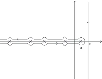
assuming absolute integrability along Resc. In the cases of interest to us, all the poles are located on the real axis to the left ofα. If the transform satisfies appropriate growth estimates, one can shift the integration contour in3.12 to run counterclockwise along the real axis from−∞toαand back,Figure 1. This reduces3.12to a sum over residues at the poles by the Cauchy residue theorem:
fx
∞
n0
Ress−γn M
fsxγn. 3.13
Ifγnare integers and the series converges,fmust be real-analytic on0,∞with at worst a pole at 0, and the residues give its Laurent coefficients at 0. For example, one can compute the Taylor expansion ofe−xat 0 using thatMe−xs: Γs,and the poles−γ
α c
Figure 1: Barnes contour for Mellin transforms.
x /0 and3.11is such a case. Under analytic assumptions that we do not reproduce here, the following weakening of3.13is still true34:
If −γn are order mn poles of (meromorphic continuation of) Mfs and its Laurent expansions at−γnhave the form
Mfs An0 sγn
An1 sγn2
mn−1 k2
Ank sγnk1
, 3.14
then an asymptotic expansion of fatx0 is
fx∼
∞
n0
An0−An1lnx mn−1
k2
−1kAnk
k! ln kx
xγn. 3.15
Now, it becomes clear where the extra 1/xin3.6came from. In addition to gamma poles in 3.11that produce terms−1n/n!ζ−nxn, there is also a simple pole ofζswith residue 1 that givesΓ1·1/x1/x. Thus,3.6is at least an asymptotic expansion ofe−x/1−e−xat 0. The fact that it actually converges to the function is a rare bonus. In general, even if3.15 does converge, it is not necessarily to the original function, see34.
This technique extends to general Fourier sumsor harmonic sumsof the form
fx
∞
k1 akg
ωkx
3.16
because their Mellin transforms can be easily expressed in terms of those of the base function
g 34. One can think of them as sums of generalized harmonics with amplitudes ak and frequenciesωk, the usual ones corresponding togx eix, ωk±k. Indeed,
Mfs
∞
k1 ak
∞
0
xs−1gω
kxdx
∞
k1 ak
ωks
∞
0
whereDs:∞k1ak/ωskis the Dirichlet series of the sum. IfDsis entire andMgsonly has simple poles ats0,−1,−2, . . . ,then
fx∼
∞
n0 Ress−n
MgsD−nxn. 3.18
If, moreover, g itself is entire and decays fast enough on R, then gx ∞n0gnxn, Ress−nMgs gn and fx∼
∞
n0gnD−nxn. The same answer can be obtained by an legitimate under the circumstancesinterchange of sums in3.16:
fx
∞
k1 ak
∞
n0
gnωkxn
∞
n0 gn
∞
k1 akωnk
xn
∞
n0
gnD−nxn. 3.19
In particular, this expansion is not just asymptotic but convergent. If Ds is not entire but only meromorphic, the last two equalities fail. However,3.15still ensures that formal interchange of sums gives the regular part of the asymptotic expansion correctly as long asD-poles are real-part positive. This is precisely what happened in3.3.
Ramanujan-Wright expansion
The situation in3.9is more complicated. We compute from3.7:
MlnMe−xs
∞
k1 1
k
∞
n1
nMe−nkxs
∞
k1 1
k
∞
n1 nΓs
nks. 3.20
Now, assume that Res is large enough for the double series to converge absolutely, for example, Res >2, and proceed
∞
k,n1 Γs
ns−1ks1 Γs
∞
n1 1
ns−1 ·
∞
k1 1
ks1 Γsζs−1ζs1. 3.21
The extra zeta poles occur ats−1, s11, that is,s0,2,ands0 becomes a double pole. Formula3.15now yields an asymptotic expansion for lnMe−xthat we state as a theorem. This is a particular case of asymptotic expansions for analytic series obtained by Ramanujan who used a rough equivalent of the Mellin asymptotics, the Euler-Maclaurin summationsee 35, Theorem 6.12. The Ramanujan considerations were heuristic and in any case remained unpublished until much later. The first rigorous asymptotic for lnMe−xis due to Wright 36. We sketch a proof for the convenience of the reader.
Theorem 3.1 Ramanujan-Wright. LetMq : ∞n11−qn−n, |q| < 1 be the MacMahon function. Then lnMe−xhas the Mellin transformMlnMe−xs Γsζs−1ζs1,Res > 2, and its asymptotic expansion atx0 alongRis
lnMe−x∼ζ3 x2
lnx
12 ζ
−1 ∞
g2
2g−1B2gB2g−2 2g−22g! x
Proof. Recall that ζs has “trivial zeros” at negative even integers 29. Poles of Γs at negative odd integers are therefore canceled by zeros of ζs−1. Analytical assumptions needed for3.15to hold are satisfied here by the classical estimates for Γand ζ29. The contributing poles are as follows.
iGamma poles ats−2,−4, . . . ,−2g, . . .with residues−12g/2g!ζ−2g−1ζ1− 2g.
iiSimple pole ofζs−1ats2 with residue 1·Γ2ζ3 ζ3.
iiiDouble pole ofΓs, ζs1ats0.
We have from the first two items and3.5
ζ3
x2
∞
g1 1
2g!ζ−2g−1ζ1−2gx
2g ζ3
x2
∞
g2
2g−1B2gB2g−2 2g−22g! x
2g−2. 3.23
To take care of the double pole, we need more than just the residue. By the well-known properties ofΓandζ,
Γ1s 1−γsOs2,
ζs 1
s−1γOs−1,
3.24
whereγis the Euler constant. Thus,
Γsζs1 Γs1ζs1
s
1
s−γOs
1
s γOs
1
s2 O1,
Γsζs−1ζs1
1
s2 O1
ζ−1 ζ−1sOs2
ζ−1
s2
ζ−1
s O1
−1/12
s2
ζ−1
s O1.
3.25
By3.15, the corresponding terms in the asymptotic expansion are lnx/12ζ−1,and it remains to combine the expressions.
Stokes phenomenon and the natural boundary
As already mentioned, the relationship betweenqand xisq eix notq e−x. Replacing formallyxby−ixin3.22, we recover the infinite sum of2.17along with three extra terms:
−ζ3
x2
ln−ix
12 ζ
−1. 3.26
How legitimate is this substitution? Had3.22been a convergent Laurent expansion, there would be no such question. But it is asymptotic and represents lnMe−x only up to exponentially small termsmore precisely, “faster than polynomially small” but we follow the standard abuse of terminology. It is well-known that such expansions depend on a direction in the complex plane in which they are taken. As one crosses certain Stokes lines originating from the center of expansion, exponentially small terms may become dominant and change the expansion drastically. This change is commonly known as the Stokes phenomenon. Moreover, for an asymptotic expansion in some direction to exist, the function must be holomorphic in a punctured local sector containing this direction in its interior. Switching fromxto−ixwhile keepingxreal positive forces us to approachqei01 along the upper arc of the unit circle, that is, along a purely imaginary direction. For an asymptotic expansion in this direction, we need to haveMqanalytically continued beyond the unit disk|q|<1. But can it be continued?
Equation3.1does not look very promising. In fact, it strongly suggests thatMq
has a singularity at each root of unity. But roots of unity are dense on the circle making it a natural boundary forMqand no analytic continuation exists. It turns out to be quite hard to turn this observation into a proof, but Almkvist shows31that ifa/bis a proper irreducible fraction, then
lnMe2πia/be−x∼ ζ3
b3x2 b
12lnxO1 3.27
for real positive x. Thus, every root of unity is indeed singular, and|q| 1 is the natural boundary.
This forces us to reconsider keeping xreal in lnMeix. Should xapproach 0 from the positive imaginary direction, we can setx iy withy > 0,and Theorem 3.1gives us an asymptotic expansion iny. We can rewrite it as an expansion inxof course as long as it is understood thatxin it is positive imaginary. This may seem like an underhanded trick but it is not. The natural domain of lnMeixis the upper half-plane, and the only distinguished direction in its interior is the positive imaginary one.
Corollary 3.2. Asymptotic expansion of lnMeixatx0 alongiR
is (taking the principal branch
of the logarithm)
lnMeix∼ − ζ3 x2
ln−ix
12 ζ
−1 ∞
g2
−1g−12g−1B2gB2g−2 2g−22g! x
2g−2
∼ − ζ3
x2 lnx
12 ζ
−1−πi
24
∞
g2
−1g−12g−1B2gB2g−2 2g−22g! x
2g−2.
Comparing this to2.17, one ought to be somewhat perplexed. If we are to take3.28 at face value thenp3t −ζ3, p1t ζ−1−πi/24?!, and there is no space for lnx/12 at all. Aside from the fact that pi-s are supposed to be homogeneous polynomials of the corresponding degree, the numbers involved are not even rational,ζ3by the Ap´ery famous result. Nevertheless, the MacMahon factor appears as is in the Chern-Simons partition function, seeLemma 5.1.
The disappearance of extra variables and appearance of irrationals suggest that some kind of averaging is involved. It would not explain lnx/12,but we may guess, that averaging ofp1t is divergent and has to be regularized giving rise to an anomalous term. Why the Donaldson-Thomas theory does not reproduce the degree zero contributions in low genus is beyond our expertise. However, from the Chern-Simons vantage point this ought to be expected. The idea of largeNduality is that the same string theory is realized on manifolds with different topology 19, 20. However, the degree zero terms in genus 0,1 are exactly the ones that record the classical cohomology of the target manifold, see 2.13. Although some relation between topologies of manifolds supporting equivalent string theories may be expected, the entire cohomology ring is certainly too much to survive a geometric transition. Therefore, these classical terms cannot enter an invariant partition function except via averages that remain unchanged by such transitions.
4. Topological vertex and partition function of the resolved conifold
This section and Section 5 are to be read in conjunction. We review the salient points of two combinatorial models, the topological vertex 12, 20, 26, 27, and the Reshetikhin-Turaev calculus 19, 37, highlighting the differences but more importantly the parallels between them. The former computes the Gromov-Witten invariants of toric Calabi-Yau threefolds, and the latter computes the Chern-Simons invariants of all closed 3 manifolds. The reason to compare them is the conjectural largeNduality between the two. Both models encode their spaces into labeled diagrams and then assign values to them according to the Feynman-like rules. However, the encoding and the rules are quite different despite intriguing correspondences. The reason why we use the topological vertex instead of just summing up2.19as in3is that it directly gives the partition function in correct variables and in an appealing form. Comparing the answer to the Chern-Simons one, it becomes reasonable to express it in a closed form via the quantum Barnes functionTheorem 5.2.
Toric webs
Just as the Reshetikhin-Turaev calculus19,37, the topological vertex is a diagrammatic state-sum model. This means that geometry of a space is encoded into a diagram, a graph enhanced by additional data, and the value of an invariant is computed by summing over all prescribed labelings of the diagram. In the Reshetikhin-Turaev calculus, the diagrams are link diagrams representing 3 manifolds via surgery37,38. In the topological vertex, they are toric webs representing toric Calabi-Yau threefolds.
(0,1)
(−1,−1)
(1,1)
(0,−1)
(−1,−1) (−1,1)
[image:21.600.186.416.96.189.2](−1,1) (1,1)
Figure 2: Toric webs ofO−1⊕ O−1and localCP1×CP1.
0
1 1
1 1
ξ
ξ1
ξ2
ξ1
ξ2
Figure 3: Toric graphs ofO−1⊕ O−1and localCP1×CP1.
O−1⊕ O−1and the localCP1×CP1i.e., the total space ofT1,0CP1×CP1are shown in Figure 2, where the primitive directions of noncompact edges are also indicated. Toric webs related by aGL2Ztransformation and an integral shift represent isomorphic threefolds. For this reason, we did not label the vertices inFigure 2, one may assume that one of them is0,0,
and all compact edges have the unit length. The toric web is a complete invariant of a toric Calabi-Yau. Indeed, the moment polytope of the torus action can be recovered from it12, 4.1and therefore the threefold itself up to isomorphism by the Delzant classification theorem 39. Analogously, a 3-manifold is recovered from its link diagram up to diffeomorphism by surgery on the link37,38. Having toric webs rigidly embedded inR2is inconvenient, one would prefer to treat them as abstract graphs, perhaps with additional data. This is possible at least as far as the topological vertex is concerned although the resulting graphs may no longer be complete invariants.
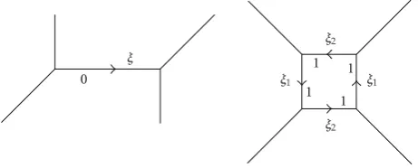
Tracing back the construction of a threefold from its web, one concludes that the vertices correspond to fixed points of the torus action and compact edges correspond to fixed rational curves copies of CP1. Being rational curves sitting inside the Calabi-Yau threefold, their normal bundles are isomorphic toOn−1⊕ O−n−1, n ±1,±2, . . . .The framing numbernefor each edgeeis assigned the value from the normal bundle type of the corresponding curve. This only determines ne up to sign, and the edge must be oriented to specify it. Although on their own these orientations are chosen arbitrarily, they must be aligned with the framing numbers, the exact rule is given in12, 4.2.
Ifξ1, . . . , ξk is an integral basis in H2X,Zas in Section 2, then each edge curveCe represents a homology class expressible as a linear combination Ce m1ξ1· · ·mkξk,
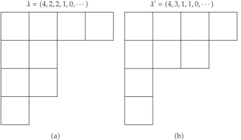
[image:21.600.186.417.231.324.2]λ 4,2,2,1,0,· · ·
a
λ 4,3,1,1,0,· · ·
[image:22.600.180.423.98.239.2]b Figure 4: Young diagram and its conjugate.
algorithmically from the web itself without any recourse to the original threefold 40, 12, 4.1.
Partitions and the Schur functions
We wish to briefly describe the topological vertex algorithm to see how q-bifactorials naturally emerge from it. This requires some basic information about partitions 8 that appear in the Reshetikhin-Turaev calculus as well. Partitions serve as labels in state sums defining the invariants. A partitionλ is an element of Z∞ with only finitely many nonzero entries that are nonincreasing, that is,
λλ1, λ2, . . . , λN,0, . . .
, λi∈Z, λ1≥λ2≥ · · · ≥λN≥0. 4.1
Let denote the set of all partitions. The number of nonzero entrieslλis called the length of a partition, and the sum of all entries|λ| : λ1 λ2 · · ·λN is called its sizeor weight. Partitions are visualized by Young diagrams, rows of boxes stacked top down withλi boxes inith row,Figure 4. The conjugate partitionλis obtained visually by transposing the Young diagram along the main diagonal and analytically asλi :max{j |λj ≥i}. Note thatλ λ andλ1 lλ, |λ| |λ|. Another relevant characteristic of a partition, sometimes called its quadratic Casimir, is
κλ:
∞
i1 λi
λi−2i1
,κλ −κλ, κλ∈2Z. 4.2
Partitions represent possible states of compact edges in a toric graph and a combination of partition labels for each edge represents a state of the graph27. The partition function is then obtained by summing over all possible states.
more technically, if monomials containing any variable outside of a finite set are discarded from the sum. For instance, if
λ 1n: ⎛
⎝1 ,1, . . . ,1 ntimes
,0, . . .
⎞
⎠ 4.3
thens1nis thenth elementary symmetric function:
s1nx enx:
1≤i1<···<in<∞
xi1· · ·xin. 4.4
In general, sλ are polynomials in the elementary symmetric functions given by the Jacobi-Trudy formulasλdeteλi−ij,1≤i, j ≤lλ λ1. For example,
s2,1,0,...x
e2 e0 e3 e1
e1e2−e0e3
∞
i1 xi·
∞
i<j1 xixj−
∞
i<j<k1
xixjxk. 4.5
Since en are homogeneous of degree n,the Jacobi-Trudy formula implies that sλ are also homogeneous of degree |λ|, that is, sλax a|λ|sλx. Moreover,sλ, λ ∈ P form a linear basis in the space of symmetric functions, in particularsλsμ ν∈Pcλμνsν. It turns out that
cλ
μνare nonnegative integers that vanish unless|ν||λ||μ|. They are the famous Littlewood-Richardson coefficients8.
Specializations of the Schur functions appearing in the topological vertex are obtained by specializing the formal variablesxito elements of a geometric series possibly modified at finitely many entries. Such specializations were extensively studied by Zhou4. Define the Weyl vectorρby
ρ:
−1
2,− 3 2, . . .
−i1
2 ∞
i1
. 4.6
Note that ρ is not a partition. Introduce a new formal variableq and for any vectorξ set
qξ: qξ1, qξ2, . . .,so, in particular,qρ q−1/2, q−3/2, . . .is a geometric series.
Definition 4.1. One-, two-, and three-point functions of the topological vertex are, respectively 4,12,
Wλq :sλqρ Wλ0q,
Wλμq:sλqρsμ
qλρ,
Wλμνq:qκμκν/2
α,β,γ∈P
cαγλ cν
γβ
WμαqWμβq
Wμ0q .
4.7
the Chern-Simons theory41. We assumeq∈C\R−andq1/2is then defined by the principal
branch of the square root. One can see by inspection from4.4thatenqλρconverges for
|q| > 1. Since the Schur “functions” sμ are polynomials inen, they are also well defined as honest functions ofqupon specializing toqλρ.
To be consistent with the usual basic hypergeometric notation42, we wish to switch from|q|>1 to|q|<1. This can be done using a symmetry of the two-point functions4
Wλμq −1|λ||μ|Wλμq−1 −1|λ||μ|sλq−ρsμ
q−λ−ρ. 4.8
This identity is a curious one since the two sides never converge simultaneouslyboth diverge for|q|1. It has the same meaning as a more familiar identity:
∞
i1
qi q
1−q −
1 1−q−1 −
∞
i0
q−i−q
∞
i1
q−i, 4.9
where the two sides never converge simultaneously either. In fact, Wλμq are rational functions of q1/2 and can be analytically continued toC\R
−, 4.8 expresses this analytic
continuation.
The appearance ofq-bifactorials in partition functions is due to the Cauchy identity for the Schur functions4,8
λ∈P
sλxsλyu|λ|
∞
i,j1
1uxiyj
. 4.10
Ifxi qi−1, yjqj−1,the right-hand side of4.10becomes
∞
i,j1
1uqi−1qj−1∞ i,j0
1uqij u;q2
∞. 4.11
Note that although4.10is a formal identity if both sides converge as in4.11, it holds as a function identity.
Partition functions as state sums
Let us now inspect the state sums appearing in the topological vertex. LetV andEc denote the sets of vertices and compact edges of a toric graph, respectively. Choose an arbitrary orientation for each element ofEc, this determines the sign of the framing numbers. Assign a formal variableai to each element of a basisξi ∈ H2X,Z,and setae : am11· · ·amkk for the corresponding edge curveCe m1ξ1· · ·mkξk. Finally, label all compact edges by arbitrarily chosen partitions λe ∈ P and noncompact ones by the trivial partition 0 ∈ P. Triples of partitions λv : λ1, λ2, λ3 are then assigned to each vertex according to the following rule.