© Hindawi Publishing Corp.
EIGENSTRUCTURE OF THE EQUILATERAL TRIANGLE.
PART III. THE ROBIN PROBLEM
BRIAN J. MCCARTIN
Received 16 June 2003
Lamé’s formulas for the eigenvalues and eigenfunctions of the Laplacian on an equilateral triangle under Dirichlet and Neumann boundary conditions are herein extended to the Robin boundary condition. They are shown to form a complete orthonormal system. Various prop-erties of the spectrum and modal functions are explored.
2000 Mathematics Subject Classification: 35C05, 35J05, 35P10.
1. Introduction. The eigenstructure of the Laplacian on an equilateral triangle under either Dirichlet or Neumann boundary conditions was explicitly determined by Lamé [6,7] in the context of his studies of heat transfer in polyhedral bodies and then further explored by Pockels [12]. However, Lamé and subsequent researchers such as Pockels did not provide a complete derivation of these formulas but rather simply stated them and then proceeded to show that they satisfied the relevant equation and associated boundary conditions. Such a complete, direct, and elementary derivation of Lamé’s formulas has only recently been provided for the Dirichlet problem [11] as well as the Neumann problem [9].
It is the express purpose of the present work to extend this recent work to the much more difficult case of the Robin boundary condition. Lamé [6, 7] presented a partial treatment of this problem when he considered eigenfunctions possessing 120◦ rota-tional symmetry. In all likelihood, Lamé avoided consideration of the complete set of eigenfunctions with Robin boundary conditions because of the attendant complexity of the transcendental equations which so arise. However, armed with the numerical and graphical capabilities of Matlab, we herein study the complete family of Robin eigen-functions of the Laplacian on an equilateral triangle.
We commence by employing separation of variables in Lamé’s natural triangular co-ordinate system to derive the eigenvalues and eigenfunctions of the Robin problem. An important feature of this derivation is the decomposition into symmetric and an-tisymmetric modes (eigenfunctions). The problem is then reduced to the solution of a system of transcendental equations which we treat numerically. Surprisingly, all of the modes so determined are expressible as combinations of sines and cosines.
(0,0) (h,0)
h 2,
h√3 2
τ r
Figure2.1. Equilateral triangle with incircle.
demonstrate orthogonality of these modes. Completeness is then established via an analytic continuation argument relying on the previously published completeness of the Neumann modes [13]. Lastly, knowing the eigenstructure permits us to construct the Robin function [1], and we so do.
2. The Robin eigenproblem for the equilateral triangle. During his investigations into the cooling of a right prism with equilateral triangular base [6,7], Lamé was led to consider the eigenvalue problem
∆T (x, y)+k2T (x, y)=0, (x, y)∈τ, ∂T
∂ν(x, y)+σ T (x, y)=0, (x, y)∈∂τ,
(2.1)
where∆is the two-dimensional Laplacian∂2/∂x2+∂2/∂y2,τis the equilateral triangle shown inFigure 2.1,ν is its outward pointing normal, and 0≤σ <+∞is a material parameter. However, he was only able to show that an eigenfunction satisfying (2.1) could be expressed in terms of combinations of sines and cosines when it possesses 120◦ rotational symmetry. We will find through the ensuing analysis that all of the eigenfunctions (modes) of this problem are so expressible.
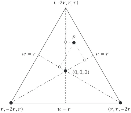
(r ,−2r , r ) (r , r ,−2r ) (−2r , r , r )
u=r
v=r w=r
p
(0,0,0)
Figure3.1. Triangular coordinate system.
Observe that in (2.1) whenσ=0, we have the Neumann problem [9] whileσ→ +∞
yields the Dirichlet problem [11]. Thus, we may profitably viewσ as a continuation parameter which provides a homotopy between these two well-understood problems. Throughout the ensuing development, we will avail ourselves of this important obser-vation.
3. Triangular coordinate system. Reconsider the equilateral triangle of sideh in standard position in Cartesian coordinates(x, y)(Figure 2.1) and define thetriangular coordinates(u, v, w)of a pointP(Figure 3.1) by
u=r−y,
v= √
3 2 ·
x−h
2
+1
2·(y−r ),
w= √
3 2 ·
h
2−x
+1
2·(y−r ),
(3.1)
wherer=h/(2√3)is the inradius of the triangle. The coordinatesu,v, andwmay be described as the distances of the triangle center to the projections of the point onto the altitudes, measured positively toward a side and negatively toward a vertex.
Note that Lamé’s triangular coordinates satisfy the relation
u+v+w=0. (3.2)
[image:3.468.128.340.68.251.2]introduced by Lamé’s contemporary Möbius in 1827 (see [3]):
U=r−u
3r , V= r−v
3r , W= r−w
3r , (3.3)
satisfyingU+V+W=1. These were destined to become the darling of finite element practitioners in the twentieth century.
4. Separation of variables. We now commence with our original, complete, and ele-mentary derivation by introducing the orthogonal coordinates(ξ, η)given by
ξ=u, η=v−w. (4.1)
Equation (2.1) becomes
∂2T ∂ξ2+3
∂2T ∂η2+k
2T=0. (4.2)
Hence, if we seek a separated solution of the form
f (ξ)·g(η), (4.3)
we arrive at
f+α2f=0, g+β2g=0, α2+3β2=k2. (4.4)
Thus, there exist separated solutions of the form
f (u)·g(v−w), (4.5)
wherefandgare trigonometric functions.
Before proceeding any further, we will decompose the sought-after eigenfunction into parts symmetric and antisymmetric about the altitudev=w(seeFigure 4.1):
T (u, v, w)=Ts(u, v, w)+Ta(u, v, w), (4.6)
where
Ts(u, v, w)=
T (u, v, w)+T (u, w, v)
2 ,
Ta(u, v, w)=
T (u, v, w)−T (u, w, v)
2 ,
(4.7)
henceforth to be dubbed a symmetric/antisymmetric mode, respectively. We next take up the determination ofTs andTa separately.
u=r
v=r w=r
v=w
Figure4.1.Modal line of symmetry/antisymmetry.
Hence, we make the ansatz
Ts=cos
π λ
3r(u+2r )−δ1
·cos
π (µ−ν)
9r (v−w)
+cos π µ
3r (u+2r )−δ2
·cos
π (ν−λ)
9r (v−w)
+cos π ν
3r (u+2r )−δ3
·cos
π (λ−µ)
9r (v−w)
,
(5.1)
with
λ+ν+µ=0, (5.2)
and eigenvalue
k2=272
π
r 2
λ2+µ2+ν2=274
π
r 2
µ2+µν+ν2. (5.3)
As we will see, this symmetric mode never vanishes identically.
Careful perusal of (5.1) now reveals that forδ1=δ2=δ3=0, it reduces to a symmet-ric mode of the Neumann problem [9], while forδ1= −3π /2,δ2=π /2, andδ3=π /2, it reduces to a symmetric mode of the Dirichlet problem [11]. Thus, our task amounts to finding values of λ, µ, ν, δ1, δ2, and δ3 so that the Robin boundary condition is satisfied along the periphery of the equilateral triangle. These values are to satisfy the constraints−3π /2< δ1≤0, 0≤δ2< π /2, 0≤δ3< π /2, 0≤µ, and 0≤ν, as well as (5.2).
Imposition of the Robin boundary condition alongu=r yields
tanλ−δ1= 3σ r
π λ , tan
µ−δ2= 3σ r
π µ , tan
ν−δ3= 3σ r
while the imposition alongv=ryields
tan
−δ2+δ3 2
=3π λσ r, tan
−δ3+δ1 2
=3π µσ r, tan
−δ1+δ2 2
=3π νσ r. (5.5)
By symmetry, the boundary condition alongw=rwill thereby be automatically satis-fied.
Introducing the auxiliary variablesL,M, andNwhile collecting together these equa-tions produces
tanλ−δ1
=tan
−δ2+δ3 2
=3π λσ r =tanL, −π2 < L≤0,
tanµ−δ2=tan
−δ3+δ1 2
=3σ r
π µ =tanM, 0≤M < π
2,
tanν−δ3
=tan
−δ1+δ2 2
=3π νσ r =tanN, 0≤N <π 2,
(5.6)
and these six equations may in turn be reduced to the solution of the system of three transcendental equations forL,M, andN:
2L−M−N−(m+n)π·tanL=3σ r ,
[2M−N−L+mπ ]·tanM=3σ r ,
[2N−L−M+nπ ]·tanN=3σ r ,
(5.7)
wherem=0,1,2, . . .andn=m,m+1, . . ..
OnceL,M, andNhave been numerically approximated, for example, using Matlab, the parameters of primary interest may then be determined as
δ1=L−M−N, δ2= −L+M−N, δ3= −L−M+N,
λ=2L−πM−N−m−n, µ=2M−πN−L+m, ν=2N−πL−M+n. (5.8)
For future reference, when m= n, we haveM =N, δ2=δ3, µ= ν, and 2π µ = δ2−δ1+2mπ.
Of particular interest are the following limits. Asσ →0+, we find thatL,M, andN each approaches 0, as doδ1,δ2, andδ3, and, most significantly,λ→ −(m+n),µ→m, andν→n. In other words, we recover in this limit the Neumann modes. Furthermore, asσ → +∞, we find that L→ −π /2, M →π /2, N→π /2, δ1→ −3π /2, δ2 →π /2, and δ3→π /2, and, most significantly,λ→ −2−(m+n),µ→m+1, andν→n+1. In other words, we recover in this limit the Dirichlet modes. Thus, we have success-fully fulfilled our original ansatz and thereby constructed a homotopy leading from the symmetric Neumann modes to the symmetric Dirichlet modes. Moreover, we have indexed our symmetric Robin modesTsm,n, which are given by (5.1) in correspondence
to the symmetric Neumann modes with the result that asσ ranges from 0 to+∞, the (m, n)symmetric Neumann mode “morphs” continuously (in fact, analytically) into the (m+1, n+1)symmetric Dirichlet mode.
σ=0.001 0
1 2 3
1
0.5
0 0
0.5 1
y x
Ts
σ=1 0
1 2 3
1
0.5
0 0
0.5 1
y x
Ts
σ=10 0
1 2 3
1
0.5
0 0
0.5 1
y
x Ts
σ=1000 0
1 2 3
1
0.5
0 0
0.5 1
y
x Ts
Figure5.1. The(0,0)symmetric mode.
σ=0.001 −2
0 2
1
0.5
0 0
0.5 1
y x
Ts
σ=1 −2
0 2
1
0.5
0 0
0.5 1
y x
Ts
σ=10 −2
0 2
1
0.5
0 0
0.5 1
y x
Ts
σ=1000 −2
0 2
1
0.5
0 0
0.5 1
y x
Ts
σ=0.001 −2
0 2
1
0.5
0 0
0.5 1
y
x Ta
σ=1 −2
0 2
1
0.5
0 0
0.5 1
y
x Ta
σ=10 −2
0 2
1
0.5
0 0
0.5 1
y x
Ta
σ=1000 −2
0 2
1
0.5
0 0
0.5 1
y x
Ta
Figure6.1. The(0,1)antisymmetric mode.
6. Construction of an antisymmetric mode. A parallel development is possible for the determination of an antisymmetric mode. In light of the oddness ofTaas a function
ofv−w, we commence with an ansatz of the form
Ta=cos
π λ
3r(u+2r )−δ1
·sin
π (µ−ν)
9r (v−w)
+cos π µ
3r (u+2r )−δ2
·sin
π (ν−λ)
9r (v−w)
+cos π ν
3r (u+2r )−δ3
·sin
π (λ−µ)
9r (v−w)
.
(6.1)
Once again,
λ+µ+ν=0,
k2= 2 27
π
r 2
λ2+µ2+ν2= 4 27
π
r 2
µ2+µν+ν2. (6.2)
However, this antisymmetric mode may vanish identically.
Equations (5.4), (5.5), (5.6), (5.7), and (5.8) still hold so that, for a givenm and n,
{λ, µ, ν, δ1, δ2, δ3} are the same for the symmetric, Tsm,n, and antisymmetric, Tam,n,
7. Modal properties. In what follows, it will be convenient to have the following alternative representations of our Robin modes:
Tm,n
s =
1 2 cos
2π
9r(λu+µv+νw+3λr )−δ1
+cos 2π
9r(νu+µv+λw+3νr )−δ3
+cos 2π
9r(µu+νv+λw+3µr )−δ2
+cos 2π
9r(µu+λv+νw+3µr )−δ2
+cos 2π
9r(νu+λv+µw+3νr )−δ3
+cos 2π
9r(λu+νv+µw+3λr )−δ1
,
(7.1)
Tm,n
a =
1 2 sin
2π
9r(λu+µv+νw+3λr )−δ1
−sin 2π
9r(νu+µv+λw+3νr )−δ3
+sin 2π
9r(µu+νv+λw+3µr )−δ2
−sin 2π
9r(µu+λv+νw+3µr )−δ2
+sin 2π
9r(νu+λv+µw+3νr )−δ3
−sin 2π
9r(λu+νv+µw+3λr )−δ1
,
(7.2)
obtained from (5.1) and (6.1), respectively, by the application of appropriate trigono-metric identities.
We may reduce the collection of antisymmetric Robin modes through the following observation.
Theorem7.1. (i)The modeTsm,nnever vanishes identically. (ii)The modeTam,nvanishes identically if and only ifm=n.
Proof. (i) Note that a symmetric mode is identically zero if and only if it vanishes
along the line of symmetryv=w since the only function, both symmetric and anti-symmetric, is the zero function. Alongv=w,
Tsm,n=cos
π (µ+ν)
3r (u+2r )−δ1
+cos π µ
3r(u+2r )−δ2
+cos π ν
3r (u+2r )−δ3
,
(7.3)
σ=0.001 −2
0 2
1
0.5
0 0
0.5 1
y x
Ts
σ=1 −2
0 2
1
0.5
0 0
0.5 1
y x
Ts
σ=10 −2
0 2
1
0.5
0 0
0.5 1
y x
Ts
σ=1000 −2
0 2
1
0.5
0 0
0.5 1
y x
Ts
Figure7.1. The(1,1)symmetric mode.
(ii) Note that an antisymmetric mode is identically zero if and only if its normal derivative vanishes along the line of symmetry v=w since the only function, both antisymmetric and symmetric, is the zero function. Alongv=w,
∂Tam,n
∂(v−w)=
π (µ−ν) 9r cos
π (µ+ν)
3r (u+2r )+δ1
+π (µ+2ν)
9r cos π µ
3r(u+2r )−δ2
−π (29µr+ν)cos π ν
3r (u+2r )−δ3
.
(7.4)
This equals zero if and only ifm=n.
Hence, our system of eigenfunctions is{Tsm,n(n≥m); Tam,n(n > m)}.Figure 7.1
σ=0.001 −2
0 2
1
0.5
0 0
0.5 1
y
x Ts
σ=1 −2
0 2
1
0.5
0 0
0.5 1
y
x Ts
σ=10 −2
0 2
1
0.5
0 0
0.5 1
y x
Ts
σ=1000 −2
0 2
1
0.5
0 0
0.5 1
y x
Ts
Figure7.2. The(0,2)symmetric mode.
σ=0.001 −2
0 2
1
0.5
0 0
0.5 1
y
x Ta
σ=1 −2
0 2
1
0.5
0 0
0.5 1
y
x Ta
σ=10 −2
0 2
1
0.5
0 0
0.5 1
y x
Ta
σ=1000 −2
0 2
1
0.5
0 0
0.5 1
y x
Ta
σ=0.001 −2
0 2
1
0.5
0 0
0.5 1
y
x Ts
σ=1 −2
0 2
1
0.5
0 0
0.5 1
y
x Ts
σ=10 −2
0 2
1
0.5
0 0
0.5 1
y x
Ts
σ=1000 −2
0 2
1
0.5
0 0
0.5 1
y x
Ts
Figure7.4. The(1,2)symmetric mode.
σ=0.001 −2
0 2
1
0.5
0 0
0.5 1
y x
Ta
σ=1 −2
0 2
1
0.5
0 0
0.5 1
y x
Ta
σ=10 −2
0 2
1
0.5
0 0
0.5 1
y x
Ta
σ=1000 −2
0 2
1
0.5
0 0
0.5 1
y x
Ta
We next give the casem=nfurther consideration. Recall that we have just deter-mined thatTam,m≡0. Furthermore, in this case, we may combine the terms of (7.1) to
yield
Tsm,m=cos
2π µ
3r (r−u)−δ2
+cos 2π µ
3r (r−v)−δ2
+cos 2π µ
3r (r−w)−δ2
,
(7.5)
which clearly illustrates that any permutation of(u, v, w)leavesTsm,minvariant. This
is manifested geometrically in the invariance ofTsm,munder a 120◦rotation about the
triangle center (seeFigure 7.1). This invariance will henceforth be termed rotational symmetry.
Moreover, the modesTsm,mare not the only ones that are rotationally symmetric.
Theorem7.2. (i)The modeTsm,nis rotationally symmetric if and only if
m≡n(≡l)(mod 3). (7.6)
(ii)The modeTam,nis rotationally symmetric if and only ifm≡n(≡l)(mod 3).
Proof. (i) The modeTsm,n is rotationally symmetric if and only if it is symmetric
about the line v=u. This can occur if and only if the normal derivative ∂Tsm,n/∂ν
vanishes there. Thus, we require that
∂Tsm,n
∂(v−u) v
=u= −
1
4 (2µ+ν)sin 2π
3r
−νu−(µ+ν)r−δ1
+(µ−ν)sin 2π
3r
(µ+ν)u+νr−δ3
−(µ−ν)sin 2π
3r
(µ+ν)u+µr−δ2
−(2µ+ν)sin 2π
3r(−νu+µr )−δ2
−(µ+2ν)sin 2π
3r(−µu+νr )−δ3
+(µ+2ν)sin 2π
3r
−µu−(µ+ν)r−δ1
=0,
(7.7)
σ=0.001 −2
0 2
1
0.5
0 0
0.5 1
y
x Ts
σ=1 −2
0 2
1
0.5
0 0
0.5 1
y
x Ts
σ=10 −2
0 2
1
0.5
0 0
0.5 1
y x
Ts
σ=1000 −2
0 2
1
0.5
0 0
0.5 1
y x
Ts
Figure7.6. The(0,3)symmetric mode.
(ii) The modeTam,nis rotationally symmetric if and only if it is antisymmetric about
the linev=u. This can occur if and only ifTam,nvanishes there. Thus, we require that
Tm,n a v=u=
1 2 sin
2π
3r
−νu−(µ+ν)r−δ1
−sin 2π
3r
(µ+ν)u+νr−δ3
+sin 2π
3r
(µ+ν)u+µr−δ2
−sin 2π
3r(−νu+µr )−δ2
+sin 2π
3r(−µu+νr )−δ3
−sin 2π
3r
−µu−(µ+ν)r−δ1
=0,
(7.8)
derived from (7.2). These terms cancel pairwise if and only if (7.6) holds.
σ=0.001 −2
0 2
1
0.5
0 0
0.5 1
y
x Ta
σ=1 −2
0 2
1
0.5
0 0
0.5 1
y
x Ta
σ=10 −2
0 2
1
0.5
0 0
0.5 1
y x
Ta
σ=1000 −2
0 2
1
0.5
0 0
0.5 1
y x
Ta
Figure7.7. The(0,3)antisymmetric mode.
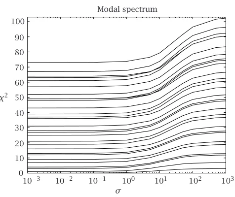
8. Spectral properties. The modal frequenciesfm,nare proportional to the square
root of the eigenvalues given by (5.3). Hence, we have
fm,n∝
4π 3hχ, χ
2:=µ2+µν+ν2. (8.1)
Thus, the spectral structure of the equilateral triangle hinges upon the properties of the spectral parameterχ2.
This spectral parameter is shown for the first 29 modes inFigure 8.1asσ ranges from 0 to+∞. The left side corresponds to the Neumann modes (σ =0) and the right side corresponds to the Dirichlet modes (σ= +∞). Thus, this figure graphically displays the homotopy relating these two well-understood eigenvalue problems.
The monotonicity of these curves is apparent and easily established from the identity
dχ2
dσ =(2µ+ν) dµ
dσ+(µ+2ν) dν
dσ ≥0 (8.2)
since(µ, ν)increase monotonically from(m, n)to(m+1, n+1)asσ varies from 0 to+∞.
SinceTsm,n and Tam,n both correspond to the same frequency fm,n given by (8.1),
Modal spectrum
0 10 20 30 40 50 60 70 80 90 100
103 102 101
100 10−1 10−2
10−3
σ χ2
Figure8.1. Spectral parameter.
intersection of two modal curves. For the Dirichlet and Neumann problems, number-theoretic techniques permit a comprehensive treatment of such spectral multiplicity [10].
[image:16.468.115.353.62.262.2]However, for the Robin problem,µandνare not integers and such techniques fail. At the present time, no general results are available and one must resort to perusal of Figure 8.1in order to locate modal degeneracies for 0< σ <+∞. All one can say with certainty is that if(m1, n1)and(m2, n2)are modal indices satisfying the inequalities
0<m22+m2n2+n22
−m21+m1n1+n21
<3m1+n1
−m2+n2
, (8.3)
then the corresponding modal curves must intersect for some value ofσ which will thereby generate a corresponding modal degeneracy.
9. Orthogonality. By Rellich’s theorem [8], eigenfunctions corresponding to distinct eigenvalues are guaranteed to be orthogonal. Also, a symmetric mode and an anti-symmetric mode are automatically orthogonal. However, as we discovered above, the multiplicity of the eigenvalues given by (5.3) is quite a complicated matter. Thus, we invoke the following continuity argument in order to confirm the orthogonality of our collection of eigenfunctions{Tsm,n(n≥m); Tam,n(n > m)}.
Suppose thatfandgare eigenfunctions of like parity that share an eigenvalue,k2, for some fixed value ofσ=σˆ. This corresponds to an intersection of two spectral curves in Figure 8.1. Forσ in the neighborhood of ˆσ, Rellich’s theorem guarantees thatf , g =
τf g dA=0. Thus, by continuity,f , g =0 forσ=σˆ and the orthogonality of our
10. Completeness. It is not a priori certain that the collection of eigenfunctions
{Tsm,n, Tam,n}constructed above is complete. For domains which are the Cartesian
prod-uct of intervals in an orthogonal coordinate system, such as rectangles and annuli, completeness of the eigenfunctions formed from products of one-dimensional coun-terparts has been established [15]. Since the equilateral triangle is not such a domain, we must employ other devices in order to establish completeness.
We will utilize an analytic continuation argument which hinges upon the previously established completeness of the Neumann modes [13]. The homotopy between the Neu-mann and Dirichlet modes that we have established above guarantees a unique branch leading from each of the Neumann modes to its corresponding Dirichlet mode. Like-wise, for any 0< σ <∞, we may trace out a branch from any mode leading back to a Neumann mode asσ→0+.
Suppose, for the sake of argument, that the collection of Robin modes constructed above is not complete for some 0< σ=σ <ˆ ∞. Then, letu(x, y; ˆσ )be a mode that is not contained in our collection. As we have a selfadjoint operator, there existanalytic branches emanating from this point in Hilbert space whereis the multiplicity ofk2(σ )ˆ [2]. Denote any of these branches, analytically continued back toσ =0 asu(x, y;σ ). Since we know that the collection of Neumann modes is complete, this branch must at some point,σ=σ∗, coalesce with a branch emanating from one of our Robin modes.
However, as we now show, the analytic dependence ofu(x, y;σ )uponσ prohibits such a bifurcation atσ=σ∗. To see this, let
∆u+k2u=0, (x, y)∈τ, ∂u
∂ν+σ u=0, (x, y)∈∂τ. (10.1)
Then
u(x, y;σ )=ux, y;σ∗+ux, y;σ∗·σ−σ∗
+ux, y;σ∗·
σ−σ∗2 2 +···,
(10.2)
whereu:=∂u/∂σand each of the correction terms in the Taylor series is orthogonal to the eigenspace ofk2(σ∗).
Each of the Taylor coefficients satisfies the boundary value problem
∆u(n)x, y;σ∗+k2σ∗u(n)x, y;σ∗=0, (x, y)∈τ, ∂u(n)
∂ν
x, y;σ∗+σ∗u(n)x, y;σ∗= −nu(n−1)x, y;σ∗, (x, y)∈∂τ, (10.3)
which may be solved recursively and uniquely foru, u, . . . , u(n), . . .since they are each
11. Robin function. Using (6.1) and (7.1), we may define the orthonormal system of eigenfunctions
φm,n
s =
Tsm,n
Tsm,n
(m=0,1,2, . . .;n=m, . . .),
φm,na =
Tam,n
Tm,n
a
(m=0,1,2, . . .;n=m+1, . . .),
(11.1)
together with their corresponding eigenvalues
λm,n=
4π2 27r2
µ2+µν+ν2 (m=0,1,2, . . .;n=m, . . .). (11.2)
Green’s function [14] for the Laplacian with Robin boundary conditions (the Robin function [1]) on an equilateral triangle is then constructed as
G(x, y;x, y)
=
∞
m=1
φm,ms (x, y)φm,ms (x, y)
λm,m
+ ∞ m=0
∞
n=m+1
φm,ns (x, y)φm,ns (x, y)+φm,na (x, y)φm,na (x, y)
λm,n
.
(11.3)
This may be employed in the usual fashion to solve the corresponding nonhomoge-neous boundary value problem [1].
12. Conclusion. In the foregoing, we have filled a prominent gap in the applied math-ematical literature by providing a complete elementary derivation of the extension of Lamé’s formulas for the eigenfunctions of the equilateral triangle to Robin boundary conditions. In addition to its innate mathematical interest, this problem is of practical interest as it relates to the calibration of numerical algorithms for approximating the eigenvalues of the Laplacian upon triangulated domains.
In addition, we have established the orthonormality and completeness of this collec-tion of eigenfunccollec-tions using the simplest of mathematical tools. Furthermore, we have made an extensive investigation of the properties of the spectrum and modes. Lastly, the Robin function has been specified.
We close with the observation that the above development is inherently dependent upon the constancy ofσ. If the eigenfunctions for variableσ were trigonometric, then that would imply that the corresponding eigenfunctions for the problem with Dirich-let/Neumann conditions along two sides of the triangle and a Neumann/Dirichlet con-dition, respectively, along the third side were also trigonometric. This would violate theorems to the contrary established in [9,11].
Acknowledgments. The author thanks Mrs. Barbara A. McCartin for her
References
[1] G. F. D. Duff,Partial Differential Equations, Mathematical Expositions, no. 9, University of Toronto Press, Toronto, 1956.
[2] K. O. Friedrichs,Perturbation of Spectra in Hilbert Space, American Mathematical Society, Rhode Island, 1965.
[3] J. Gray,Möbius’s geometrical mechanics, Möbius and His Band (J. Fauvel et al., ed.), Oxford University Press, New York, 1993.
[4] K. Gustafson and T. Abe,The third boundary condition—was it Robin’s?Math. Intelligencer 20(1998), no. 1, 63–71.
[5] ,(Victor) Gustave Robin: 1855–1897, Math. Intelligencer20(1998), no. 2, 47–53. [6] G. Lamé,Mémoire sur la propagation de la chaluer dans les polyèdres, Journal de l’École
Polytechnique22(1833), 194–251 (French).
[7] , Leçons sur la Théorie Analytique de la Chaleur, Mallet-Bachelier, Paris, 1861 (French).
[8] C. R. MacCluer,Boundary Value Problems and Orthogonal Expansions. Physical Problems from a Sobolev Viewpoint, IEEE Press, New Jersey, 1994.
[9] B. J. McCartin,Eigenstructure of the equilateral triangle. II. The Neumann problem, Math. Probl. Eng.8(2002), no. 6, 517–539.
[10] ,Modal degeneracy in equilateral triangular waveguides, J. Electromagn. Waves Appl.16(2002), no. 7, 943–956.
[11] ,Eigenstructure of the Equilateral Triangle, Part I: The Dirichlet Problem, SIAM Rev. 45(2003), no. 2, 267–287.
[12] F. Pockels,Über die partielle Differentialgleichung∆u+k2u=0, B. G. Teubner, Leipzig, 1891 (German).
[13] M. Práger,Eigenvalues and eigenfunctions of the Laplace operator on an equilateral triangle, Appl. Math.43(1998), no. 4, 311–320.
[14] G. F. Roach,Green’s Functions, 2nd ed., Cambridge University Press, Cambridge, 1982. [15] W. A. Strauss,Partial Differential Equations, An Introduction, John Wiley & Sons, New York,
1992.
Brian J. McCartin: Department of Applied Mathematics, Kettering University, 1700 West Third Avenue, Flint, MI 48504-4898, USA