GOLD PRICE FORECASTING IN INDIA USING ARIMA MODELLING

GE-International Journal of Management Research

© Associated Asia Research Foundation (AARF)

Website: www.aarf.asia Email : [email protected] , [email protected]

GOLD PRICE FORECASTING IN INDIA USING ARIMA MODELLING

Aarti Mehta Sharma1 and Saina Baby

Symbiosis Institute of Business Management, Bangalore-560100

Symbiosis International University

ABSTRACT

Historically, gold has been identified as a unique commodity because of its ability to act as a

hedge against inflation and its stability during periods of financial volatility and crises. Tracing

the trends in Gold prices and conducting a price forecast is relevant from the point of view of

Gold producers, investors and various central banks in the world. Time series analysis is a

popular forecasting method for predicting the future value of variables. Time series forecasting

techniques attempt to account for changes in the variable over time by examining trends. This

technique also uses historical data to predict the future value of a variable. The objective of this

study was to develop a suitable forecasting model for the price of gold. ARIMA (Autoregressive

Integrated Moving Average) model has been used in this paper for Gold price forecasting. Data

pertaining to monthly average gold prices from the RBI website for the time period April 1990 –

July 2015 were used to develop a suitable forecasting model on SPSS. Stationarity was checked

through the Augmented Dickey Fuller test and through charts. The best fit was identified by

examining various statistics and the forecasting errors.

KEYWORDS

Gold prices, Time Series, forecasting model, ARIMA , SPSS, forecasting errors, Augmented

Dickey Fuller test,best fit.

INTRODUCTION

Gold is a unique commodity because of its store of value potential and investment asset status. It

long as the world economy remains uncertain and investors feel inflation and sovereign default,

gold will keep its allure (The Economist – July8, 2010).Its ability to act as a hedge against

inflation and the use of Gold as a component of a country‟s official forex reserve makes it the

most sought after commodity in the world. At a macro-level, forecasting gold price has a lot of

applications in emerging markets. Bullish trends are expected for gold, for buildup of massive

amount of debt. The move by central banks to buy Gold in recent years plus recent pick-up in

physical flows from West to East is evidence to support to this. Tracing the trends in Gold prices

and conducting a price forecast is relevant from the point of view of Gold producers, investors

and various central banks in the world. Being the second largest consumer of Gold in the world,

75% of Gold demand in India has taken the form of jewellery in the last decade (World Gold

Council). The seasonal nature of jewellery demand plays a very important role in forecasting

Gold prices.

There has been more than 600% increase in price of Gold between 2001 and 2011.During this

period price of Gold had gone up to $1923 per ounce. But from 2012 onwards Gold prices

started declining from $1900 an ounce to $1200 an ounce. This was mainly due to better

economic conditions, low interest rates and investors‟ preference towards better performing

assets. This declining trend was continuing in 2013 also. Since Gold prices are influenced by

factors like value of dollar, opportunity cost of holding Gold, inflation and deflation, hedging

and de-hedging activities, central bank purchases, jewellery and investor demand, futures

market, supply conditions etc, changes in external environment creates volatility in Gold price

movements.

Forecasting – the art or science of predicting the future - is an integral aspect of business

management as it helps in decision making and forward planning. But the existence of dynamic

and uncertain business environment makes forecasting a highly complex and challenging

function of analytics. Forecasting, especially commodity price forecasting is an essential activity

which is helpful in analysing the demand supply dynamics existing in a market. There are several

forecasting techniques, one of them being Time series data forecasting. Time series data are data

gathered on a given characteristic over a period of time at regular intervals. Time series

forecasting techniques attempt to account for changes over time by examining patterns, cycles,

like graphing the data to using simple averages, moving averages, weighted moving averages,

smoothing, regression analysis, ARIMA modelling etc.

Most time series data are composed of four components – Trend, Seasonality, Cyclicality and

Irregular components. Trend is defined as the long term general movement of data. Cycles are

patterns of highs and lows through which data move. Seasonal effects are shorter cycles

measured over months or quarters. They are generally measured over a year. Irregular

fluctuations are rapid changes which are unexplained for e.g. Changes in trend due to riots or

other unforeseen circumstances. Time series data that contain no trend, cyclicality or seasonality

effects are said to be stationary.

Gold price forecasting using Time series analysis is well supported in the literature. While a

number of papers are available on predicting the gold price using different time series

techniques; most of them are done in the foreign context. India specific studies are very limited.

The present research work is an attempt to fill this research gap. The study has a lot of

applications in emerging countries like India. When concerned with investment options,

developed markets behave differently than emerging markets. In emerging markets where

interest rates are below inflation rates and where there is a growing middle class with greater

disposable income investment in gold is a very good option for savers to hedge against inflation.

This coupled with cultural factors increases the demand for Gold in countries like India.

The objective of this study was to develop a suitable forecasting model for the price of gold. For

this purpose monthly average gold prices from the RBI website for the time period February

1990 – September 2014 were used.

The major hypothesis in analyzing the price oscillations in different markets (goods, stocks

financial markets, etc.) is the accidental nature of the market. We know that one of the reasons of

gold price change is the external effects such as economic policies, environmental conditions and

cultural factors. One general assumption made in such cases is that the historical data incorporate

all those behaviour. As a result, the historical data is the major input to the prediction process.

There are several forecasting techniques available; those are developed mainly based on different

assumptions, mathematical foundations and specific model parameters. However, for better

results, it is important to find the appropriate technique for a given forecasting task. We have

error and come to a final conclusion about the model which best fits the fluctuation in the gold

market and best predicts gold prices. In this, we found that the ARIMA(0,1,1) works best.

LITERATURE REVIEW

This section provides a brief overview of the existing literature about gold price forecasting.

Rebecca Davis,et.al(2014) in their paper “Modeling and Forecasting of Gold Prices on Financial Markets” have conducted a study on Gold price forecasting using ARIMA model. Monthly

adjusted price of Gold during the period January 2003 to April 2012 was used for analysis. The

fitted ARIMA model was used for a six step ahead forecast. The forecasted values were

compared with the actual to understand forecasting accuracy.

Gangopadhyay,Kausik.et.al(2014) in their paper “Forecasting the price of gold: An Error

Correction Approach” have tried to identify the long term relationship of Gold price with

factors like exchange rate,US Bond rates,oil prices, consumer price index and stock market index

using Vector Error Correction model. Since the time series variables in the study were

non-stationary, the authors have done the analysis in a co integrating approach using Vector error

correction model provided by Johansen and Juselius.

Aye,Godness et,al (2014) in their working paper titled „Forecasting the Price of Gold Using Dynamic Model Averaging‟ attempted to examine the possible factors influencing the price of

Gold.Thorugh the analysis of data the authors tried to show superiority of the dynamic model

averaging (DMA) and dynamic model selection (DMS) models over Bayesian model averaging

and linear models. Based on the study it was identified that exchange rate factor and Fed‟s

financial stress index have more impact on the gold prices than any other variables. It was also

revealed that the exchange rate factor has the maximum impact of the gold prices.

Hossein Hassanix_,Emmanuel Sirimal Silvax and Rangan Gupta(2014) in their working paper “Forecasting the Price of Gold” made a comparison of the predictive power of 17 existing

forecasting methods. The study was based on Gold price data obtained from www.kitco.com for a period from January 1972 to December 2013.Based on the results, the authors arrived at the

horizons. But,if we consider lowest average Root Mean Square Error as the criterion for judging

the predictive power of a amodel,Exponential Smoothing(ETS) will be the best model.

Lili,Li and Diao Chengmei(2013) in their paper used Factor-Augmented Vector

Auto-regression(FA VAR) model to predict gold prices. The authors have classified all major factors

influencing gold prices(Y) into three principal components- gold reserve and prices of energy

products ( F1 ), financial market indices( F2 ), global macroeconomic indicators( F3 ).Through

analysis of data from 1985 to 2005 it was identified that there was a positive relationship

between F1 and Y negative relationships between F2 and Y and also between F3 and Y.

Dr.Ali Khan,Massarrat M(2013) has done a study on Gold Price Forecasting using Box Jenkins

Auto Regressive Integrated Moving Average (ARIMA) Approach. His study aimed at building a

model for Gold price forecasting and developing a framework for checking the accuracy of the

model. The study was based on sample data of Gold price( in US$ per ounce) during the period

January 2003 to March 2012.For building the forecasting model, the study has used Box Jenkins

Auto Regressive Integrated Moving Average(ARIMA) method. After comparing the results from

ARIMA(0,1,1) and ARIMA(1,1,0) models it was identified that ARIMA(0,1,1) is a more

suitable forecasting model for Gold Price Forecasting. Forecasting Accuracy of the model was

tested using Root Mean Square Error, Mean Absolute Error and Mean Absolute Percentage

Error.

Abdulla,Lazim(2012),conducted a study using ARIMA model to forecast gold prices. This study

was done in the context of Malaysian economy by taking daily selling Malaysian gold coin

prices from 2002-2007.This study was mainly conducted with the objective of assessing the

investment potential of Gold coins. As the forecasted gold coin prices using the ARIMA showed

an upward trend, investment in gold coin is justified by the identified long term trends. Based on

the study they arrived at the conclusion that ARIMA model is not suitable for making gold price

forecasting because of the influence of too many factors on gold prices.

M.G Deepika, Gautam Nambiar and Rajkumar M (2012) in their paper identified that the short

run and long run gold prices exhibited diverging trends.Thereofore they used two different

forecasting was done using time series modeling and long run price forecast using multiple

regression analysis.Thier study was based on the gold price data for the period from 1980 to

2012.Based on their study they arrived at the conclusion that ARIMA is not a suitable model for

predicting gold prices.Therfore they have use the multiple regression model to analyse the

influence of various factors in deciding gold prices. Through this analysis they identified three

major factors which influenced the gold prices – worls stock prices,US$ index and inflation.

Anand Ashesh and Piyush Dharnidharka(2012) in their paper carried out a study about

forecasting gold prices using time series analysis. They have used Box - Jenkins methodology to

forecast the monthly average gold prices. Monthly average gold price data for the period January

2012 to June 2012 was taken for analysis. According to them, though many new models are used

to make accurate forecasts in the long run, ARIMA models are still useful in making short term

forecasting mainly because of the fair degree of precision which was identified in their study.

Shafiee,Shahriar and Erkan Topal(2010) developed a model for Gold price forecasting by using

historical gold prices from January 1968 to December 2008.This model identified three

components which were very important in influencing the gold price movements. These were

long-term trend reversion component, diffusion component and jump/dip component. Long-term

trend reversion component explain the tendency of gold prices to revert to the historical long

term trend. The diffusion component defines a range for the random variations in gold prices

compared to the long term historical trend. Based on analysis of data this random variation range

was calculated as 25% which means that the gold price in the next month will increase or

decrease by 25% compared to the long term trend. The dip/jump component explains the

deviation of gold prices from the long term trend by more than 25%.The influence of these three

components was validated with historical gold prices and the model was used to predict the gold

price for next 10 years.

Ismail,Z et,al (2009) carried out Gold price forecasting using Multiple Linear Regression

method. MLR was done with London PM Fix Gold Prices as the dependant variable and

Inflation Rate,Money supply,Dollar-Euro exchange Rate,NewYork Stock Exchange

Bill and UD Dollar Index as independent variables. Forecasting using MLR generally leads to

two major problems – multicollinearity and correlated error terms. The issue of multicollinearity

was addressed in this study by the using step wise regression method and it reduced the number

of independent variables to four. Prais-Winsten procedures were employed in the study to

address the second problem of correlated error terms.This forecasting model using MLR finally

identified four major factors influencing future Gold prices - CRB index, EUROUSD exchange

rate, inflation rate and money supply (M1).

DATA AND METHODOLOGY

Data pertaining to monthly average gold prices from the RBI website for the time period April

1990 – July 2015 were used to develop a suitable forecasting model. There were a total of 304

cases starting from April 1990 – July 2015. The maximum value of gold was INR 31672.83

corresponding to September 2012 and the minimum was INR 3284.70 corresponding to July

1990. The mean value was 10487 and the standard deviation was 8886. The measures of

skewness and Kurtosis were well within ± 3.

We used the Box-Jenkins methodology(ARIMA process) to find the best fit. Autoregressive

Integrated Moving Average model is generally knows as ARIMA(p,d,q) model where p denotes

the number of autoregressive terms, d the number of times the time series has to be differenced

before it becomes stationary and q the number of moving average terms. ARIMA model is used

for analysing a times series which shows non stationarity.Non stationarity can be removed by

differencing the time series. Non stationarity was measured through sequence charts and The

Methodology

Exploratory Data Analysis &Checking for Stationarity

Transforming and differencing

Model Identification(s)

Best fit

Forecasting

We measured the forecasting errors through Mean Absolute Error (MAE), Root Mean Square

Error (RMSE).Mean Square Error (MSE) and Mean Absolute Percentage Error (MAPE).

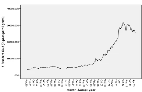
Figure 1: Exploratory Data Analysis : Sequence Chart

Stationarity can be defined in precise mathematical terms, but for our purpose we mean a

flat looking series, without trend, constant variance over time, a constant auto correlation

structure over time and no periodic fluctuations.

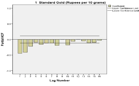
We checked the data for stationarity by checking for autocorrelation and partial

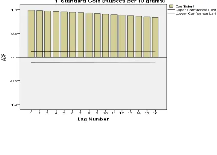
autocorrelation as well as through the ADF test. Figure 1 shows us that the data is not

stationary and this is further corroborated by the ACF and PACF charts shown below in

Figure 2 and 3. These show us that the data is not stationary.

The p value for the Augmented Dickey Fuller test was 0.83 which also proves that the data

is non stationary.

Figure 2:Auto Correlation Function (ACF)

Figure 3:Partial Auto Correlation Function (PACF)

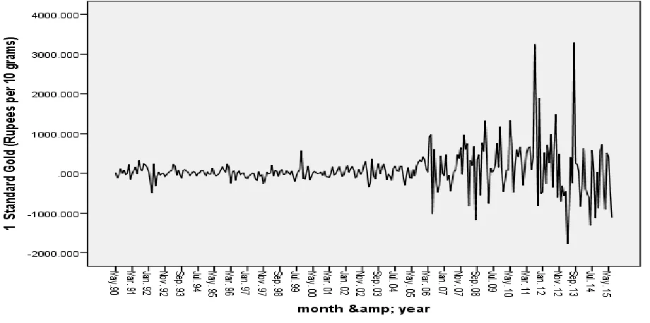
We then transformed data by differencing once and checked for stationarity.

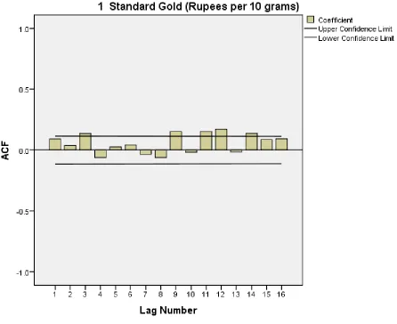
Figure 5:Auto Correlation Function (ACF) (Differencing Once)

Figure 7: Exploratory Data Analysis : Sequence Chart (Differenced twice)

Figure 9:Partial Auto Correlation Function (PACF) (Differenced twice)

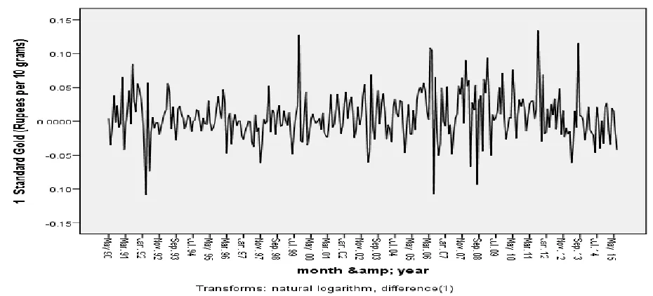
Figure 10: Exploratory Data Analysis : Sequence Chart (Natural log transformation and

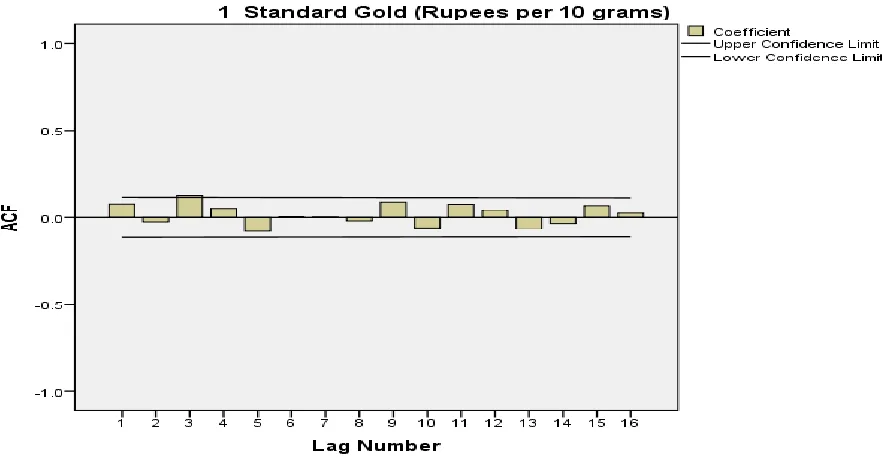
Figure11:Auto Correlation Function (ACF) (Natural log transformation and differenced

once)

Figure 12:Partial Auto Correlation Function (PACF) (Natural log transformation and

The p value for the Augmented Dickey Fuller test was 0.01 which proves that the data has

become stationary

Figure 13: Exploratory Data Analysis : Sequence Chart (Natural log transformation and

differenced twice)

LOGTRANSFORMED AND DIFFERENCED TWICE

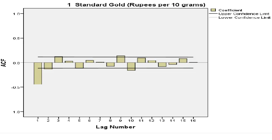
Figure 14:Auto Correlation Function (ACF) (Natural log transformation and differenced

Figure 15:Partial Auto Correlation Function (PACF) (Natural log transformation and

differenced twice)

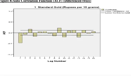
By examining the data through figures 1 to 15 we conclude that the data is stationary BY

DIFFERENCING ONCE AND LOG TRANSFORMING. The ADF for that is also 0.01 proving

that the data is now stationary. After making the data stationary, we tried identifying the best fit

model using ARIMA modeller in SPSS and came out with the following models which fitted the

Mo del No Model (p,d,q non seasonal ) (p,d,q seasonal) Lju ng-Box Q

BIC R

squa

red

RMS

E

MAE MA

PE Foreca st for Septem ber 2015 Lower Control Limit@ 5% Upper Control Limit@ 5%

1 (0,1,0)(0,

0,0)

0.23

3

12.4

17

0.997 492.1

85 282.40 4 2.53 3 25911.0 41 23531.0 62 28465.0 68

2 (0,1,0)(0,

1,0)

0.00

0

13.0

36

0.994 670.8

01 406.79 6 3.63 6 24618.6 57 21512.4 74 28045.7 49

3 (0,1,1)(0,

0,0)

0.15

8

12.4

31

0.997 491.0

25 281.84 7 2.51 4 25810.4 33 23345.2 80 28463.5 97

4 (0,0,0)(0,

1,0)

0.00

0

15.3

09

0.945 2089.

538 11300. 838 10.8 40 29601.8 60 22468.0 43 38291.7 99

5 (0,1,2)(0,

0,0)

0.15

2

12.4

54

0.997 492.1

69 281.17 9 2.50 8 25877.7 61 23398.0 76 28547.2 34

Actual value for gold on September 15, 2015 is Rs.24,550 (Source:

http://www.goldpricesindia.com )

Of all the five models which fitted the data, model numbers 1,3 and 5 were a good fit. On

examining the statistics, Model number 3 which is an ARIMA with non seasonal p=0,d=1 and

q=1 fits the data the best as the BIC(Bayesian Information Criterion) is low and RMSE,MAE

and MAPE are the least. As the Ljung Box Q is greater than 0.05,it shows that autocorrelations

for one or more lags might be significantly different from zero which indicates that the values are

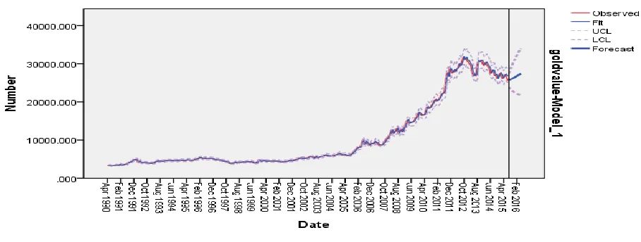
Figure 16: Model Fit

CONCLUSION

In this study of a univariate time series based on monthly Gold prices starting from April 1990 to

July 2015, we used the standard gold price (22k) of the Mumbai market. We have examined the

data and applied a log normal transformation and a differencing of one to make it stationary. We

have used SPSS to fit various ARIMA models to the data. We find that the ARIMA(0,1,1) is the

best fit for the said data (as shown in Figure 16). This model can be used to estimate the price of

gold in the future.

FUTURE SCOPE:

There is scope for further research wherein the model can be applied using daily gold price data.

BIBLIOGRAPHY

1. Abdullah ,Lazim.((2012). ARIMA Model for Gold Bullion Coin Selling Prices

Forecasting. International Journal of Advances in Applied Sciences (IJAAS).Vol: 1, No:

4, December 2012.Pages: 153-158.

2. Aye,Godness et,al(2014). Forecasting the Price of Gold Using Dynamic Model

Averaging. University of Pretoria Department of Economics Working Paper Series.

3. Anand Ashesh and Piyush Dharnidharka.(2012).Forecasting God Prices using Time

Series Analysis.

http://www.academia.edu/2960558/Forecasting_Gold_Prices_using_Time_Series_Analys is (accessed on October 2014).

4. Gangopadhay,Kausik.et.al(2014). Forecasting the price of gold: An Error Correction

Approach. Working paper,IIMK/WPS/155/ECO/2014/13.Indian Institute of

Management,Kozhikode.Pages 1-15.

5. Gaynor, Patricia E and Kirkpatrick Rickey C. (1994) .Introduction to Time Series

Modeling and Forecasting in Business and Economics. Tata McGraw - Hill International

USA.

6. Greene, William H. (2003). Econometrics Analysis. Fifth Edition. Pearson Education Inc

USA.

7. Gujrati, Damodar N. (2004) .Basic Econometrics. Fourth Edition. Tata McGraw - Hill

International USA.

8. Hassani, Hossein, Emmanuel Sirimal Silva and Rangan Gupta.(2014). Forecasting the

Price of Gold. IPAG Business School Working Paper,Pages: 1-15.

9. Ismail, Z., Yahya A. And Shabri A. (2009) ' Forecasting Gold Prices Using Multiple

Linear Regression Method'. American Journal of Applied Sciences. Volume: 6.Pages:

1509-1514.

10.Khan Ali, (2013), Forecasting of gold prices (Box Jenkins Approach). International

Journal of Emerging Technology and Advanced Engineering, 662 -668.

11.Lili,Li and Diao Chengmei.(2013). Research of the Influence of Macro-Economic

12.M.G Deepika, Gautam Nambiar and Rajkumar M. (2012). Forecasting Price and

Analyzing Factors Influencing The Price Of Gold Using ARIMA Model And Multiple

Regression Analysis. International Journal of Research in Management, Economics and

Commerce. Volume: 2 Issue: 11. Pages: 548-563.

13.Rebecaa,Davis et.al(2014). Modeling and Forecasting of Gold Prices on Financial

Markets.American Internaional Journal of Contemporary

Research,Volume:4,Number:3.Pages 107-113.

14.Shafiee,Shahriar and Erkan Topal.(2010). An overview of global gold market and gold