Online Decision Support System and Machine Learning Modeling using Bayesian Belief Network

Online Decision Support System and Machine Learning

Modeling using Bayesian Belief Network

S.Karpagaselvi

Research Engineer,

Pentagram Research Center Private Limited, Hyderabad, AndraPradesh, India.

M.Thiyagarajan

LEJ Brouwer School of Intutionstic Logic, Pentagram Research Center Private Limited,

Hyderabad, AndraPradesh, India.

ABSTRACT

In this study we investigate the use of Bayesian Belief Networks (BBN) for developing a practical framework for machine learning process incorporating the commonsense reasoning. Bayesian Belief Networks grant a systematic and localized method for structuring probabilistic information about a situation into coherent whole. Bayesian networks have been established as a ubiquitous tool for modelling and reasoning under uncertainty. In this study we attempt to develop a graphical model that is used to represent knowledge about the uncertain domain in which the nodes are the random variables and the edges between the nodes represent probabilistic dependencies among the corresponding random variables. These conditional dependencies in the graph are often estimated by using some known statistical and computational methods. Thus developed Bayesian belief network along with joint probability distribution in the factored form can be used to evaluate all possible inference queries both predictive and diagnostic by marginalization. We experimentally developed a model for educational institutions which could be used to take decision on considering various factors link campus placement, total cost per year, academic excellence etc.

General Terms

Bayesian Belief Network, Decision Support system

Keywords

Bayesian Belief Network, Marginalization, Joint Probability, Conditional Probability, Machine Learning , Node Probability Table

1.

INTRODUCTION

1.1 Bayesian approach

Bayesian probability is a formalism that allows us to reason about beliefs under conditions of uncertainty. Suppose „a‟ is a statement „Institution X will get full admission in the next Academic Year‟ is an event with uncertainty. Every individual may have different beliefs in the statement depending on their specific knowledge of factors that might effect its likelihood. Raman may have a strong belief in the statement „a‟ based on his knowledge of the current and past data of admissions. Soman on the other hand, may have a much weaker belief in the statement based on some of his specific knowledge of knowing a new world class institution „Y‟ is being started in the next academic year in the nearby location of X.

Thus, in general, a person's subjective belief in a statement „a‟

as P(a|K). Raman's belief in „a‟ is different from Soman's because they are using different K's. However, even if they were using the same K they might still have different beliefs in „a‟.The expression P(a|K) thus represents a belief measure and calculated using bayes theorem Equation (1) .

P(a│ K) = P(K│a)P(a) / P(K) (1)

1.2 Bayesian network

Bayesian probability is a formalism that allows us to reason about beliefs under conditions of uncertainty. A Bayesian network, Bayes network, belief network or directed acyclic graphical model is a probabilistic graphical model that represents a set of random variables and their conditional dependencies via a directed acyclic graph (DAG) which is representating the probabilistic relationships between parent node and child node. Given evidence, the network can be used to compute the probabilities of the events represented by the nodes. A Bayesian network for a set of variables X = (X1,X2,...Xn) consists of

(1) a network structure S that encodes a set of conditional independence assertions about variables in X, and

(2) a set P of local probability distributions associated with each variable.

Together, these components define the joint probability distribution for X. The network structure S is a directed acyclic graph. The nodes in S are in one-to-one correspondence with the variables X. We use Xi to denote both the variable and its corresponding node, and Pai to denote the parents of node Xi in S as well as the variables corresponding to those parents. Conditional independencies between the nodes are encoded with the lack of possible arcs in the S. In particular, given structure S, the joint probability distribution for X is given by

p(x) = ∏(p(xi │ pai ) 1<i<n (2)

The local probability distributions P are the distributions corresponding to the terms in the product of Equation 2. Consequently, the pair (S, P) encodes the joint distribution p(x).

Bayesian network represent conditional dependencies between the nodes connected by the edge. Nodes which are not connected represent variables which are conditionally independent of each other. Each node is associated with a probability function that takes as input a particular set of values for the node's parent variables and gives the probability of the variable represented by the node. For example, if the parents are Boolean variables then the probability function could be represented by a table of entries, one entry for each of the possible combinations of its parents being true or false.

Efficient algorithms exist that perform inference and learning in Bayesian networks. Bayesian networks that model sequences of variables are called dynamic Bayesian networks. Generalizations of Bayesian networks that can represent and solve decision problems under uncertainty are called influence diagrams.[2]

1.3 Pearl's Bi-directional Belief Updating

Algorithm

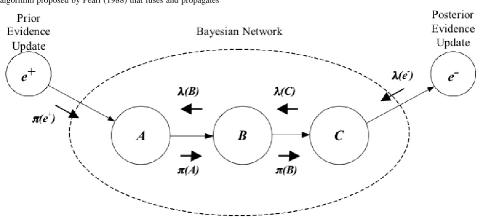
One of the most powerful characteristics of Bayesian Networks is its ability to update the beliefs of each random variable via bi-directional propagation of new information through the whole structure. This was initially achieved by an algorithm proposed by Pearl (1988) that fuses and propagates

the impact of new evidence providing each node with a belief vector consistent with the axioms of probability theory. The figure 1 below shows a graphical representation of Pearl's bi-directional propagation scheme. Roughly speaking, information can be inserted in Bayesian

Networks through a data updating in the prior probabilities or in the posterior probabilities. In the first case, the new data will flow via a π row vector (prior evidence vector), while in the former case data will flow via a λ column vector (posterior evidence vector). Both vectors update the node belief (say node B) by the equation:

.

(3)

where “α” is a normalizing constant, and “ • “ means term by term multiplication (inner or dot product). The resulting column vector is the new belief of node B, clearly, vector Bel(B) will have as many elements as the number of states of the random variable depicted by node B.

Figure 1 Graphical representation of Pearl's bi-directional propagation scheme

Nodes of a Bayesian network have different number of states, which will reflect in the number of elements each π or λ vectors will have. After receiving a π vector with updated information from a parent node (say A), node B will send its own π vector to its children nodes. The equation used in node B for creating its π vector is:

(4)

(5) where the resulting column vector λ(B) is then transmitted to parent nodes.

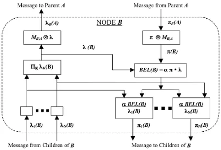
When a node has multiple children, which means it may receive different λ vectors. The node internal algorithm must be able to deal with these vectors concurrently, as more than one node can send λ vectors at the same time. The figure 2 below shows the internal structure of a single node processor, which explains how this problem was solved by Pearl's algorithm. [1][8]

Figure 2 Internal structure of a single node processor

The Evidence is of two types

 Hard evidence or Instantiation for a node X is evidence that the state of X is known definitely.

 Soft evidence for a node X is any evidence that enables us to update the prior probability values for the states of X.

Types of connection in a BBN have a strong influence on transmission of evidence in the Bayesian Network. Three different types of connection are existing in BBN and how the evidence is propagated in the different connections are explained below.

Serial connection

In serial connection any evidence entered at the beginning of the connection can be transmitted along the directed path providing that no intermediate node on the path is instantiated (which thereby blocks further transmission). In a serial connection from B to C via A, evidence from B to C is blocked only when we have hard evidence about A.

Diverging connection

In diverging connection a parent node has more than one child node. Any evidence can be transmitted between two or more child nodes of the same parent providing that the parent is not instantiated. In a diverging connection where B and C have the common parent A evidence from B to C is blocked only when we have hard evidence about A.

Converging connection

Definition of d-separation:

Two nodes X and Y in a BBN are d-separated if, for all paths between X and Y, there is an intermediate node A for which either:

1. The connection is serial or diverging and the state of A is known for certain; or

2. The connection is converging and neither A nor any of its descendants have received any evidence at all.[1]

2. RELATED WORK

Norman Fenton and Martin Neil (2011) shows how the Bayesian network approach helps to identify, understand and quantify the complex interrelationships (underlying even seemingly simple situations) and can help us make sense of how risks emerge, are connected and to represent the control and mitigation of them. By thinking about the hypothetical causal relations between events they investigated alternative explanations, weigh up the consequences of the actions and identify unintended or undesirable side effects.[3]

Nir Friedman and Moises Goldszmidt suggest unsupervised learning of Bayesian networks for classification tasks.The Experimental validation of the tree of tree augmented naive Bayesian classifiers could be used in machine learning community.

Pearl‟s algorithm performs exact Bayesian updating, but only for singly connected networks. Subsequently, general Bayesian updating algorithms have been developed. One of the most commonly applied is the Junction Tree algorithm (Lauritzen & Spiegelhalter, 1988). Neapolitan (2003) provides a discussion on many Bayesian propagation algorithms. Although Cooper (1987) showed that exact belief propagation in Bayesian Networks can be NP-Hard, exact computation is practical for many problems of practical interest.

Some complex applications are too challenging for exact inference, and require approximate solutions (Dagum & Luby, 1993). Many computationally efficient inference algorithms have been developed, such as probabilistic logic sampling (Henrion, 1988), likelihood weighting (Fung & Chang, 1989; Shachter & Peot, 1990), backward sampling (Fung & del Favero, 1994), Adaptive Importance Sampling (Cheng & Druzdzel, 2000), and Approximate Posterior Importance Sampling (Druzdzel & Yuan, 2003).

Several researchers have developed probabilistic inference algorithms for Bayesian networks with discrete variables that exploit conditional independence roughly as we have described, although with different twists. For example, Howard and Matheson (1981), Olmsted (1983), and Shachter (1988) developed an algorithm that reverses arcs in the network structure until the answer to the given probabilistic query can be read directly from the graph. In this algorithm, each arc reversal corresponds to an application of Bayes' theorem.

Pearl (1986) developed a message-passing scheme that updates the probability distributions for each node in a Bayesian network in response to observations of one or more variables. Lauritzen and Spiegelhalter (1988), Jensen et al. (1990), and Dawid (1992) created an algorithm that first transforms the Bayesian network into a tree where each node in the tree corresponds to a subset of variables in X. The algorithm then exploits several mathematical properties of this tree to perform probabilistic inference. Most recently,

In1991, developed an inference algorithm that simpli_es sums and products symbolically, as in the transformation from Equation 21 to 22. The most commonly used algorithm for discrete variables is that of Lauritzen and Spiegelhalter (1988), Jensen et al (1990), and Dawid (1992).

Methods for exact inference in Bayesian networks that encode multivariate-Gaussian or Gaussian-mixture distributions have been developed by Shachter and Kenley (1989) and Lauritzen (1992), respectively. These methods also use assertions of conditional independence to simplify inference. Approximate methods for inference in Bayesian networks with other distributions, such as the generalized linear-regression model, have also been developed (Saul et al., 1996; Jaakkola and Jordan, 1996).

3. SYSTEM OVERVIEW

Here we are proposing a decision support system based on the Bayesian Belief Network, which would respond for the queries by supplying the known facts, partial facts, evidence, requirements etc. This is graphical model of the educational institutions, which would aid us to identify our requirement are met by an institution say „C1‟. This is a new direction of using dynamic programming for search application.This decision Support system would be embedded in any hand held systems like mobile phones, or on any embedded systems which will be used by the students to identify an institution of their needs and interest among the competitors.

This kind of models could be used in online search, with and effective information retrieval system which retrieves the required evidence for the given query from world wide web and identify the answers for the queries. This kind of models could be employed in the web crawlers, for indexing which improves the ranking scheme based on contents of the sites instead of merely the page hits.

3.1 Bayesian Network Constructions

The Construction of the Bayesian belief Network based on two observations

 People can often readily assert causal relationships among variables. Causal relationships typically correspond to assertions of conditional dependence. The causal semantics of Bayesian networks are in large part responsible for the success of Bayesian networks as a representation for expert systems

 The Final step of Construction of Bayesian Belief Network is assessing the local probability distributions by the equation 2.

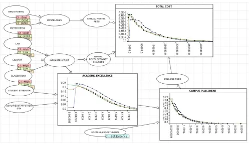
In particular, drawing arcs from cause variables to their immediate effects results in a network structure that satisfies the definition of Bayesian Belief Network. The important and main thing to start with the construction of the Bayesian Belief network is determining the variables of the model. One Possible choice of the variables for our Problem is Total Annual cost per student, Campus placement, annual development charges, hostel facility, Hostel fees, Academic Excellence ,Infra structure, Labarotory, Library, classrooms, student strength, Quality staff strength, Department etc. Obviously the real model will also include much more variables like Accreditations, Affiliation, Branches, Alumina are under development. The next step is assessing the local probability distribution of the Nodes.

 Correctly identify the goals of modeling (e.g., prediction Total cost per student per Year, Campus Placement etc),

 Identify many possible observations that may be relevant to the problem (e.g., Hostel Facilities, Qualified Staff strength, Class room , lab etc)

 Determine what subset of those observations is worthwhile to model (e.g., Hostel Facilities will increase the Hostel fees, Hence Hostel fees is a dependent variable of the hostel facility).

 Organize the observations into variables having mutually exclusive and collectively exhaustive states. (e.g., Hostel facilities having the states Best, better and Good, infra structure is a dependent variable of the Lab, Library and class room) In the next phase of Bayesian-network construction, we build a directed acyclic graph that encodes assertions of conditional independence by the equation 2 for all the nodes in the Graph

model. The construction of Bayesian networks that does not require an ordering of variables. The approach is based on two observations:

 Pople can often readily assert causal relationships among variables,

 Causal relationships typically correspond to assertions of conditional dependence.

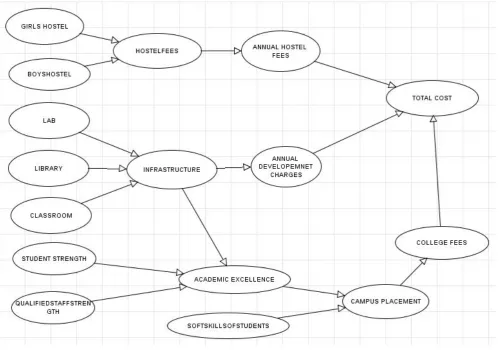
In particular, to construct a Bayesian network for a given set of variables, we simply draw arcs from cause variables to their immediate effects. In almost all cases, doing so results in a network structure that satisfies the definition. The next phase of construction is assessing the local probability distribution of the network which is stored in table called Node probability table. Figure 3 A graphical Model used for experimental purpose is shown. All the model used is constructed by the AgenaRisk tool.[4]

Figure 3 An Experimental Bayesian Belief Network for Educational Institution

3.2 Node Probability Table

The NPTs capture the conditional probabilities of a node, given the state of its parent nodes. Every node in a BBN has an associated Node Probability Table. If node A has parent nodes B and C then the NPT for node A expresses the probability p(A|B,C) for all possible combinations of A, B and C. If A has x states, B has y states and C has z states then the NPT has xyz cells.

Table 1. Probability of the hostel facility.

HOSTEL BEST BETTER GOOD

BOYS HOSTEL

0.2 0.6 0.2

GIRLS HOSTEL

0.1 0.7 0.2

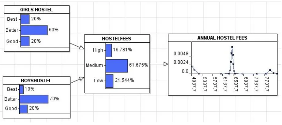
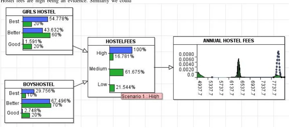
The Node probability table for the HOSTELFEES is given Table 2. It captures the conditional probabilities of the hostel fees given for all condition of the girl‟s hostel and boy‟s hostel. From the table it is evident that the probability of the hostel fees being high is 90 percent, if both girls hostel and boys hostel provides the best facilities.

Similarly all the nodes Node Probability tables are constructed based on the previous observations or by identifying the mean, median variance of a normal distribution. Some of the variables will have discrete states or some continuous variables could be modeled as discrete variables for simplicity . Few variables needs to be modeled as continuous variables essential like Hostel Fees , academic Excellence etc for finer course of decision with more number of states. The Node Probability table for this continuous variable is given by the probability distribution functions.

The main use of BBNs in Decision support systems is requirement of statistical inference needed. In addition to statements about the probabilities of events, the user knows some evidence, that is, some events that have actually been observed, and wishes to infer the probabilities of other events, which have not as yet been observed. Using probability calculus and Bayes theorem it is then possible to update the values of all the other probabilities in the BBN. This is called propagation. Bayesian analysis can be used for both 'forward' and 'backward' inference.

Figure 4. Simple Bayesian Network Model for Hostel fees Table 2 : Node probability Table for HOSTEL FEES

3.3 Evidence and Propagation in Bayesian

network

The most important use of BBNs is in revising probabilities in the light of actual observations of events that is evidence.For example if we are sure that the Hostel fees is high for an institution „X‟ then we can use this observation to determine the

a. The probability of the girls hostel facility is best

b. The probability of the girls hostel facility is better c. The probability of the girls hostel facility is good d. The probability of the boys hostel facility is best e. The probability of the boys hostel facility is better f. The probability of the boys hostel facility is good To calculate this we use the Bayes theorem. The probability of the Girls Hostel facility being high for the known evidence of Hostel fee is high is calculated by the equation 3,4,5 and thus providing an inference for the observation. When we HOSTEL

FEES

GIRLS HOSTEL

BEST BETTER GOOD

BOYS HOSTEL

BEST BETTER GOOD BEST BETTER GOOD BEST BETTER GOOD

HIGH 0.90 0.50 0.1 0.5 0.1 0.0 0.1 0.0 0

MEDIUM 0.1 0.5 0.8 0.5 0.8 0.5 0.8 0.5 0.1

enter evidence and use it to update the probabilities is called propagation. Figure 5 shows the updated probabilities when Hostel fees are high being an evidence. Similarly we could

achieve all the predications of the given evidence for all the nodes in Bayesian Belief Network.

Figure 5 Updated Probabilities of both Girls and boys hostel for given evidence of Hostel fee is high.

3. 4 Inference in a Bayesian Network

Once we have constructed a Bayesian network from prior knowledge, data, or a combination, it is usually needed to determine various probabilities of interest from the model. For example, in our problem concerning Academic institutions, we want to know the probability of Total annual Cost per student, Academic Excellence and Campus Placement etc given observations of the other variable like student strength, lab , library , hostel facilities etc. This probabilities are not stored directly in the model, and hence needs to be computed. In general, the computation of a probability of interest given a model is known as probabilistic inference. Explanation of probabilistic inference in Bayesian networks is beyond the scope of the article. Interested readers may refer to [1].

4 . RESULTS AND DISCUSSIONS

Figure 6. Risk table supplied with Query and Evidence

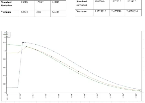
Figure 7 Prediction of Total annual Cost per student for 3 different Institutions C1,C2 &C3.

Table 3 Prediction of Total annual Cost per student for 3 different Institutions C1,C2 &C3.

Table 4 Prediction of Academic Excellence of 3 different Institutions C1,C2 &C3.

Parameters C1 C2 C3

Mean 145520.0 153050.0 166030.0

Median 116400.0 105570.0 118850.0

Standard Deviation

108270.0 155720.0 163340.0

Variance 1.1723E10 2.425E10 2.6678E10

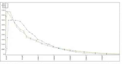
Figure 8 Prediction of Academic Excellence of 3 different Institutions C1,C2 &C3.

Parameters C1 C2 C3

Mean 3.4657 2.6215 2.8194

Median 3.0866 2.2283 2.4433

Standard Deviation

1.9605 1.9647 2.0082

Figure 10 Predicted output for the given scenario

Table 5 Prediction of Campus Placement for 3 different Institutions C1,C2 &C3

5. FUTURE DIRECTIONS

The Experimental model will be elaborated with additional variable to have more accurate prediction. Such fine models are embedded in hand held devices and could be used for making decision with the data available as facts and evidence. This kind of models could be used in online search, with and effective information retrieval system which retrieves the required evidence for the given query from world wide web and identify the answers for the queries. This kind of models could be employed in the web crawlers, for indexing which improves the ranking scheme based on contents of the sites instead of merely the page hits.

6. REFERENCES

[1] Pearl J, 'Probabilistic reasoning in intelligent systems' Morgan Kaufmmann, Palo Alto, CA, 1988.

[2] Fenton, N.E. and M. Neil, „Risk Assessment with Bayesian Networks‟ publication 2012, London: Chapman and Hall.

[3] Norman Fenton and Martin Neil „The use of Bayes and casual modeling in decision making, uncertainty and risk „ white paper 2011

[4] AgenaRisk 2010, http://www.agenarisk.com

[5] Fenton NE, Neil M, and Caballero JG, Using ranked nodes to model qualitative judgments in Bayesian Networks. IEEE Transactions on Knowledge and Data Engineering 19(10), 1420-1432 (2007).

[6] David Heckerman‟ A Tutorial on Learning With Bayesian Networks‟ a technical report on Microsoft MSR-TR-95-06 Microsoft Research Advanced Technology Division Microsoft Corporation One Microsoft Way Redmond, WA 98052.

[7] Pazzani M.J „ Searching for dependencies in Bayesian classifiers „ In Proc of the 5th

Int Workshop on artificial intelligence and statistics

Parameters C1 C2 C3

Mean 1.2 1.3664 1.4586

Median 0.91147 0.90051 0.99137

Standard Deviation

1.0469 1.5086 1.5565