Experimental Study of Temperature Control using Soft
Computing
Nithya
Venkatesan
School of Electrical Engineering VIT University , Chennai Campus , TamilNadu,
India,
N.Sivakumaran
Department of Instrumentation and Control Engineering,
National Institute of Technology, Tiruchirapalli,
TamilNadu, India
P.Sivashanmuguham
Department of Chemical Engineering, National Institute of Technology, Tiruchirapalli,
TamilNadu, India
ABSTRACT
This paper experimentally investigates the control of an industry based shell and tube heat exchanger. The hot fluid outlet temperature in the shell side is maintained by manipulating the cold fluid temperature in the tube side. The Fuzzy Logic based Controller (FLC) has been implemented in a MATLAB environment using cost effective ADAM’s module and compared with the Proportional - Integral (PI) controller. The performance of the controller has been investigated for multiple changes in set points and load changes. The fuzzy logic based controller has higher speed of response and the steady state error for the fuzzy logic control has a small average value than that of the PI control. There is less oscillatory behavior with the fuzzy logic controller, which allows a system to reach steady-state operating conditions in regions where PI controller is not able to perform well. The time domain specifications like rise time, settling time, overshoot and the performance indices, Integral Squared Error (ISE) and Integral Average Error (IAE) have been compared to PI controller.
Keywords: Nonlinear System, Shell and Tube Heat Exchanger, PI Controller, Fuzzy Logic Controller.
1. INTRODUCTION
According to the law conservation of energy, “Energy can neither be created nor destroyed but it can be transformed from one form to other”, and after all types of energy transformation and utilization it gets converted in the form of heat. The transfer of heat is one of the most basic unit operations in the process industries. Heat can be transferred between the same phases (liquid to liquid, gas to gas) or phase change can occur either in the process side (condenser, evaporator, and reboiler) or in the utility side (steam heater) of the heat exchanger. Heat exchangers are extremely complex devices for which the prediction of their operation is virtually impossible. The complexity of these systems is that due to their geometrical configuration, the physical phenomena present in the transfer of heat and to the large number of variables involved in its operation. The control problem of heat exchanger is rather difficult due to its nonlinear dynamics and particularly to the variable steady state gain and the time constant with the flow rate of the process fluid.
The use of traditional PI controllers may require several tuning adjustments for a satisfactory performance. A large number of contributions, dealing with the control of the temperature distribution for the heat exchanger, is available in the literature .Katayama et al.[1] discussed an optimal tracking control of a heat exchanger with load change. They derived a state-space model of a heat exchanger, using an
ARX model to the open-loop data obtained from the process. Their paper deals with the properties of the tracking control algorithm and are analyzed by both simulation studies and experimental studies. Their studies show that the controller performance implemented using PID proves to be the better for load changes. Xia et al. [2] have discussed about the two different control schemes for a parallel flow heat exchanger. Model reduction techniques are applied to obtain low-order models that are suitable for dynamic analysis and controller is design based on the simulation studies.
Davison et al. [3] have discussed about the dynamics and control of a polymer film compact heat exchanger. It was found that the responses of the model to disturbances in inlet temperatures could be controlled well using a digital form of PI control. Chidambaram and Malleswararao [4] proposed a model reference nonlinear controller for a temperature control of process fluid in a fluid – fluid heat exchanger. This proposed nonlinear controller shows more robust performance than that of a partial linearization controller and the design procedure of this controller is also easier. Dugdale and Wen [5] have discussed the improved controller performance of an ammonia/steam heat exchanger by optimizing the existing PID controllers. A suitable optimization schemes that could be applied to the existing control hardware, a 'feed forward' with 'dynamic decoupling' strategy was proposed.
Fuzzy control is well indicated in all the situations and provides a reasonable and effective alternative to classical controllers when the system model becomes complex and inaccurate, and does not allow us to an exact description without mismatch FLC techniques have found many successful applications and demonstrated significant improved performance. Skrjanc et al. [6] have presented a fuzzy adaptive cancellation control and compared it with model - reference adaptive control. The comparison has been made by implementing the above for a heat exchanger and it proves to be superior to classical model - reference adaptive control. Fischer et al.[7] have applied a fuzzy model based predictive controller to the temperature control of an industrial - scale cross - flow water / air heat exchanger.
response and the steady state error has a smaller average value than that of the PID control. Maidi et al. [10] have studied the control of heat exchanger, described by a partial differential equation, by optimizing a linear PI fuzzy controller. Through simulation they proved that the performance of the heat exchanger gives better results for a fuzzy controller in comparison with the traditional controller.
In this work, real time model is designed for controlling the hot fluid temperature in a shell and tube heat exchanger. The process model is experimentally determined from step response analysis and is interfaced to real time with MATLAB using simple cost effective ADAM’s module. The controller tuning model is accomplished using Fuzzy logic controller and the performances are compared with Skogestad’ s based PI controller settings based on performance indices like Integral Squared Error(ISE) and Integral Average Error(IAE).
2. REAL - TIME EXPERIMENTAL
SETUP
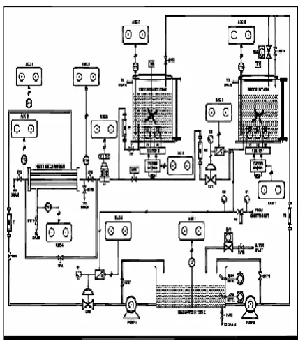
The schematic of shell and tube heat exchanger setup used in the present study is shown in the Figure 1. This has two fluids streams which can flow in both co-current and counter- current mode. The hot fluid flows from the process tank and passes through the tubes of the heat exchanger. Heater1 heats the fluid in the process tank to particular operating temperature. Cold fluid flows from the reservoir tank into the shell side of the heat exchanger. The objective of this work is to maintain the hot fluid outlet temperature by varying the cold fluid inlet rate.
[image:2.595.320.534.68.313.2]The experimental setup consists of a shell and tube heat exchanger, with suitable facilities to have both co-current and counter current flow of liquids. It also has two DPT’s connected to orifice to measure the flow rates of two streams, two I/P converters so as to regulate the air in two control valves connected to the two inlet streams. Apart from this there are six RTD’s to measure the temperature in process tank, disturbance tank, hot water inlet and outlet, cold water inlet and outlet. There are two thyristor drives which are used to regulate the voltage and current in the heater banks to regulate the process and the disturbance tanks. All the sensors and actuators are interfaced with ADAM’s module which in turn is connected to the PC through RS - 232 serial port. The DPT 1 and DPT 2 are connected to the orifice to measure the inlet flow rate of the two streams and at the same time hot water inlet temperature is measured with RTD and the cold water flow rate is changed through I/P converter which is actuated by the control action given by the controller algorithms. The manipulated variable ,cold water flow rate, is varied through the change in control valve opening which is caused by the change in air pressure (3 - 15 psi) supplied from the I/P converter when actuated by (4 - 20 mA) by the controller to achieve the set point of hot water outlet temperature which is the controlled variable. Figure 2 shows the experimental setup interfaced with ADAM’s module. Table 1 gives the technical specifications of the experimental setup.
[image:2.595.317.540.364.645.2]Figure 1 Schematic Representation of Experimental Setup
Table 1: Technical specifications of heat exchanger setup
Heat Exchanger
Type Shell and Tube in
Co-current and Counter Co-current mode
Shell material SS 316
Tube material Copper
Tube length 750mm
Shell diameter 150mm
Number of Tubes 37
Pitch Triangular 15 mm
Passes Single
Tube Diameter 6 mm
PID Controller
Input 24 V
Output 4 - 20 mA
Temperature Sensor
Sensor PT - 100, 3-wire
Transmitter 4 - 20mA/0 - 5V
Thyristor Power Controller
Load Current 20A max.
Load Voltage 150 V - 260V AC
Load Type Constant
Resistance Heater Load
Auxiliary Power 85 - 265V AC
Minimum Load Current 0.6A
Control Input 4 - 20mA
Output Continuously
Variable
Power Supply Unit
Input 230 V , 50Hz AC
Output 24 V 500mA DC
Hot Water Control Valve
Spring range 0.2-1 kg/cm2
Trim size ½”
Characteristics Equal percentage
Valve action Air to open
Cold Water Control Valve
Spring range 0.2 - 1 kg/cm2
Trim size ½”
Characteristics Equal percentage
Valve action Air to close
PUMP
Flow Rate 360L/hr Max
RPM 20 - 250RPM
I/P converter
Input 4 - 20 mA
Output 0.2 - 1 bar
Pressure Gauge
Range 0 - 30 psi
Differential Pressure Transmitter (DPT)
Input 10.5 V- 45 V
Output 4 - 20 mA
Measuring 2.5 – 250 mbar
Heater
Power Rating 1.5 KW
Supply 230 V, 50 Hz
Rotameter
Range 0 - 150 lph
Range 0 - 300 lph
3. MODEL IDENTIFICATION
3. 1 Mathematical Modeling
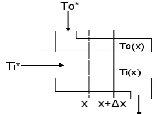
Figure 3 Single phase shell and tube Heat Exchanger
Hot water with inlet temperature Ti* and Cold water with inlet temperature To* enter the tube and shell side of the heat exchanger respectively as shown in the Figure 3. The overall heat transfer coefficient is U.
Applying the energy conservation law to each fluid we get,
0
)
T
T
(
d
U
dx
dT
C
W
i pi i
i
o
(1)0
)
T
T
(
d
U
dx
dT
C
W
o po o
i
o
(2)Rearranging the above equations and solving for Ti:
0
)
(
2
i i o
i
D
T
T
D
(3)where pi i i
C
W
d
U
,
x
d
d
D
,po o o
C
W
d
U
Roots of the equation
0
)
(
2
r
r
o
i (4)are:
0
r
,r
(
o
i)
Complementary solution:x i i i i o
e
C
B
x
T
(
)
( ) (5) Similarly x o o o i oe
C
B
x
[image:3.595.341.511.120.238.2]The constants in the above equations are related as follows:
Bi = Bo (7)
Ci = o
o i
C
(8)
On solving Eq (7.6) and Eq (7.7) we get:
1 *
*
1
o
T
To
Bo
i
(9)
1 *
1
o i
T
Co
(10)
where
T
*
Ti
*
To
*The equation (4) is a quadratic equation representing the nonlinearity involved in heat exchanger. The equations 6 and 7 indicate the variation of temperature of cold water and hot water stream along the length of the tube and when the flow rates are constant then these equation can also be used to represent the variation with respect to time.
3.2 Black Box Modeling
Here in real time implementation, system identification of this nonlinear process is done using black box modeling. For a fixed hot water inlet temperature of 50 0C and a flow rate of 50 lph the cold water flow rate was kept at 50 lph. The hot water outlet temperature was initially at 34.53 0C. Suddenly a step change is introduced and the hot water inlet flow rate is increased to 70 lph in about 220 secs. Then the corresponding hot water outlet temperature are noted until it reaches a steady state value which in this case is 44 0C. The model is further validated, it is observed that the model replicates the process well and the average error is found to be ±1.5 %.
Using the Sundaresan and Krishnaswamy [11] method, the parameters of FOPDT transfer function model and by using the experimental data the transfer function found to be
287.48
0.4905
( )
376.54
1
s
e
G s
s
(11)4. DESIGNING OF PI CONTROLLER
After deriving the transfer function model, the controller is to be designed for maintaining the system to the optimal set point. This is achieved by properly selecting the tuning parameters
K
P and
I for a PI controller. According to themethod proposed by Skogestad’s [12] the PI controller settings are
1
C c
p
K
K
(12)
I
(13) By following the Skogestad settings [64], the values foundare,
Kc
1.3352
I
376.54
and then used in real time PI Controllersettings
5.
DESIGN
OF
FUZZY
LOGIC
CONTROLLER
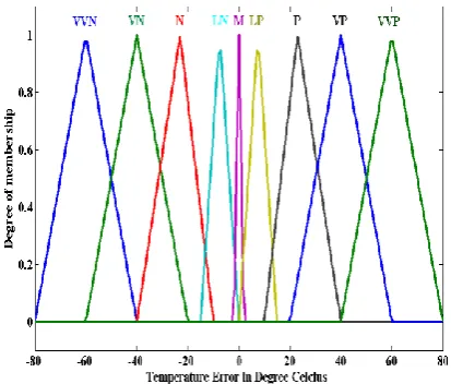
The fuzzy controller is designed with two input variables, Error(E), Change of error(CE) and one output variable as current to I/P converter which in turn will vary the position of control valve (CV) thus changing the flow rate of the cold water. The universe of discourse for E, CE and CV is scaled from 20 to 100˚C, -80 ˚C to +80˚C and 4 to 20 mA respectively. The fuzzy membership functions are defined using the triangular function equation. The triangular membership function defined for E, CE and CV output is shown in Figures 4 to 6. The fuzzification scheme employed is MIN - MAX and the defuzzification is done by using the method of heights.
[image:4.595.318.525.514.690.2]Figure 4 Membership function for Error (E)
Figure 6 Membership Function of Control Valve(CV)
6. RESULTS AND DISCUSSIONS
Both the FLC and traditional PI controllers were designed, implemented and tested for the various set points. The graphs for servo responses for both fuzzy and PI controller are shown in Figures 7 to 9.
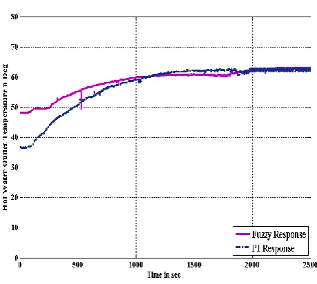
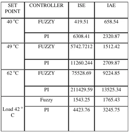
[image:5.595.319.532.75.246.2]Initially for the set point of 40 0 C the plant is run under the co current mode and then the set point is changed to 49 0C and subsequently to 62 0 C. From the Fig 7.11 to 7.13, it is clear that the FLC responses immediately to the set point changes. It is found that the FLC follows the steady state without oscillations and overshoot. The tracking of the set point change in a FLC is good compared with the Skogestad’s conventional PI Controller. Suddenly a load disturbance is introduced by increasing the hot water inlet flow for about five minutes and the response is noted and is illustrated in Figure 10. From Figure 10, it is also clear that fuzzy controller tracks the set point quickly without any oscillations. This is also validated by the performance indices values which are shown in Table 7.2 for various set points.
[image:5.595.317.538.79.489.2]Figure 7 Servo Response for 40 0C
[image:5.595.315.545.282.488.2]Figure. 8 Servo Response for 49 0C
Figure 9 Servo Response for 62 0C
[image:5.595.56.290.494.658.2] [image:5.595.318.536.538.712.2]Table 7.2 Performance indices comparison
7. CONCLUSION
It is found for hot fluid temperature control in a shell and tube heat exchanger for all set point and load changes, the performance of the intelligent controller is much superior compared to the conventional PI controller. The FLC provides a satisfactory response when compared with conventional PI controller. The FLC was able to keep the process parameters in the optimum range whenever the set point and load change occurred in real time. This is also validated by the ISE and IAE values.
8. ACKNOWLEDGEMENT
The authors would like to thank the Department of Instrumentation and Control Engineering, National Institute of Technology, Tiruchirapalli, and TamilNadu, India for carrying out this real time work in the Instrumentation & Control Laboratory.
9. REFERENCES
[1].Katayama ,T., Ithoh, T., Ogawa,M., and Yamamoto, H., 1990.Optimal tracking control of heat exchanger with change in load condition, Proc. of 29th IEEE conference on Decision and Control , 3, 1584 - 1589 .
[2].Xia, L., De Abreu-Garcia, J.A., and Hartley, T.T., 1991.Modeling and simulation of a heat exchanger, IEEE conference on Systems Engineering, 453 – 456 . [3].Davidson, G., Jachuck, R. J., Tham, M. T., and Ramshaw,
C., 1995.Heat Recovery Systems and CHP, 15(7), 609 - 617 .
[4].Chidamabaram, M., and Malleswararao, Y.S.N., 1992.Non-linear controllers for a heat exchanger, J. Proc. Contr., 2(1), 17 - 21 .
[5].Dugdale, D., Peng Wen.,2002. Controller optimization of a tube heat exchanger, Intelligent Control and Automation, Proc of the 4th World Congress, 54-58 . [6].Igor Skrjanc., Katarina Kavs .,Ek-Biasizzo Drago Matko ,
1999.Real-time fuzzy adaptive control ,Engineering Applications and Intelligence , 10(1), 53 – 61.
[7].Fisher ,M., Nelles,O., and Isermann, R.,1998. Applications to industrial processes, Control Engineering Practice , 6(2), 259 - 269 .
[8].Ibrahim, R., Othman, M.I., and Baharudin , Z., 2004.Empirical Modelling and Fuzzy Control Simulation of a Heat Exchanger, Proc of Intelligent Systems and Control , 446.
[9].Kapil Varshney and Panigrahi, P.K., 2005.Artificial neural network control of heat exchanger in a closed flow air circuit, J. of Applied Soft Computing , 5, 441 - 465. [10].Ahmed Maidi., Moussa Diaf., and Jean Pierre Corriou
2007.Optimal linear PI fuzzy controller design of a heat exchanger , Chemical Engineering and Processing . [11].Sundaresan, K.R., and Krishnaswamy, R.R.,
1978.Estimation of time delay, Time constant parameters in Time, Frequency and Laplace Domains, Canadian Journal of Chem.Eng., 56, 257 .
[12].Bruyne, F.De., 2003.Iterative feedback tuning for internal model controllers, Control Engineering Practice ,11, 1043 - 1048 .
SET POINT
CONTROLLER ISE IAE
40 oC FUZZY 419.51 658.54
PI 6308.41 2320.87
49 oC FUZZY 5742.7212 1512.42
PI 11260.244 2709.87 62 oC FUZZY 75528.69 9224.85
PI 211429.59 13525.34
Load 42 o C
Fuzzy 1543.25 1765.43