Aggregate import demand function for Pakistan: a co integration approach

Munich Personal RePEc Archive

Aggregate import demand function for

Pakistan: a co-integration approach

Iqbal, Javed and Tahir, Muhammad and Baig, Mirza Aqeel

Karachi University

10 March 2001

Online at

https://mpra.ub.uni-muenchen.de/23756/

Proc. Eighth Stat. Sem. 2001. K.U.

lSBN-969-8397-07-8-(2

SRQPONMLKJIHGFEDCBA

I7-224)

FEDCBA

A G G R E G A T E I M P O R T D E M A N D F U N C T I O N F O R P A K I S T A N :

A C O - I N T E G R A T I O N A P P R O A C H

J a v e d I q b a l , M u h a m m a d T a h i r a n d M i r z a A q e e l B a i g

RQPONMLKJIHGFEDCBA

D e p a r t m e n t o f S t a t i s t i c s . K .u .. G o v t . C o l l e g e o f C o m m e r c e & E c o n o m i c s . K a r . a n d C o l l e g e o f B u s i n e s s M a n a g e m e n t . K a r a c h i

A B S T R A C T

This paper examines the determinants of aggregate import demand for Pakistan for the period

1972-1999. The Johansen (1988) co-integration analysis is used for establishing a long run relationship

between real imports and its determinants namely real GDP, relative prices and exchange rate

volatility. The error correction model is used to capture possible short run disequilbrium. This study

provides evidence of a unique long run import demand function. This is further supported by analyzing impulse response function and variance decomposition.

I . I N T R O D U C T I O N

!

I

I

The empirical literature lacks studies on import demand determinants for developing countries

as indicated by Gafar (1988), Sarmad (1989) etc. This paper provides an evidence of import function

for Pakistan. This work differs from other studies for Pakistan in that no study has yet emerged that

exploits the time series econometric techniques of co-integration, error correction, vector

autoregression. impulse response function and variance decomposition analysis. Additionally, since

real imports and its major determinants such as real output, relative prices and exchange rate volatility

are non stationary, any evidence without considering the co-integration of the variables leads to

inappropriate use of classical t and F-tests, as explained in Granger and Newbold (1974), Fuller

(1985), Dickey and Fuller (1979,1981), Engle and Granger (1987), Phillips and Perron (1988),

Johansen (1988.1991) and Johansen and Juselius (1990). Presence of non-stationary variables in time

series regression leads to (i) non- normal coefficient distribution (ii) spurious regression problem (iii)

inconsistent and inefficient ordinary least square estimates of parameters (iv) Invalid error correction

representation.

Gafar( 1998) specified import as function of real income (real GDP) and relative prices(ratio of

import prices to CPI) for the period 1967-84 for Trinidad and Tobago. Results show that income

elasticity is more than one and price elasticity is less than one but has a positive sign. Sarmad (1989) specified import as function of real income (real GNP) relative prices (ratio of import prices to whole sale price index adjusted for level of terriff) and foreign exchange reserves for Pakistan for the period

1959-86. The function was estimated in both aggregated and disaggregated form. The study indicates

that income elasticity lies between 1.537 to 1.419 and relative price elasticity lies between 1.146 to -1.20.

Following this introduction the paper is organized as follows. Section 2 provides theoretical

foundation and modeling of import function. Variable definition and data source appear in section 3.

2. THE MODEL

Using parameter notation from Johansen and Juselius (1990), a vector autoregression model of

order k is specified as

Y,

=

RQPONMLKJIHGFEDCBA

1 l + 1 CIY,-1 + ···+ 1 C kY,-k + I / > X , +£,

SRQPONMLKJIHGFEDCBA

t

=

1,2 ... , T (2.1)

Where Y , is a p dimensional vector of endogenous variables. X, is a vector of exogenous variables,

e , is the usual error correction term such that £,-NID(O,~). 1C₁,1 C2 , ••••,1 Ck are pxp matrices of

parameters that contain the coefficients of endogenous variables. I/> contains coefficient of exogenous.

variables and J..I is vector of constants. Due to non-stationarity of most economic time series, the V AR

in (2.1) is expressed in first difference form with an error correction term to save valuable long run

information as:

(2.2)

Where

r j =-(/-1C₁ - 1 C2 - •••••••••• -1Cj ) ,

1 C= - ( / - 1 C I - 1 C2 - •.•••• - 1 Ck )

i = 1,2 ... , k-l

(2.3)

The Johansen co-integration method consists of testing the rank of zrto establish the number of

co-integrating vectors. Following three possible cases may arise

(I) Rank of 1 C= 0, i.e. 1Cisa null matix.

FEDCBA

I n this case traditional methods of regression on first

difference V AR are appropriate and no error correction representation is required.

(II) Rank of 1 C= P i.e. 1Cis full rank matrix, in this case a VAR in level is suitable since each y , is

stationary at level.

(III) Rank of 1 C= r <p i.e. 1 C is not a full rank matrix. I n this case the coefficient matrix can be written

as

1 C=a{3'

Where a and (3are each matrices of dimension P x r. The eigenvalues Aj (i=I,2, .... p) of the matrix 1 C

are computed and the test statistics developed by Johansen (1988) is used.

p

A -Trace(r) = - T

L

log(l- Aj )

j=r+l

(2.4)

This statistic is to test the hypothesis that there are at most r co-integrating vectors against the

alternative that the number is more than r. Another test statistic:

A - Max(r, r+ 1)= -T log(l-

A

r+1) (2.5)

This is used to test the hypothesis that there are r co-integrating vectors against the alternative

In our case, the vector

RQPONMLKJIHGFEDCBA

Y , consists of real imports and its determinants i.e.

Y!

=

(M,G,RP,V)' . Where M is real import, G is real output, RP is relative price and V is exchange

rate volatility, which in this case, is constructed as a four year moving standard deviation as:

3

~ A

SRQPONMLKJIHGFEDCBA

2

V

=

L J ( R , _ i - R , - i ) 1 4

i=O

(2.6)

Where R, is nominal exchange rate (Rupees/dollar) and R , is its fitted value obtained using ARIMA

model.

In functional form the import demand function is specified as

M

=

f(G, RP. V)

This model is consistent with Arize and Shwiff( 1998) for G-7 countries. They specified import

as function of real GDP, relative prices(ratio of unit value index of import to CPI) and exchange rate

volatility. The normalized co-integration vectors shows that income elasticity is more than unity, price

elasticity is negative and less than one and coefficient of exchange rate volatility is al 0negative and

less than one in magnitude.

Pakistan adopted managed float exchange rate system in 1982, earlier exchange rates were

pegged so a dummy variable (DUM) war; used as an exogenous variable to capture this change but

subsequently it was dropped since it came out to be insignificant.

Economic theory asserts that the sign of the partial derivatives are as follows:

at

>0

at

< 0

at

< 0

a G 'aRP , a V

A log linear function form is specified since it is backed by considerable empirical support e.g. Sarmad

(1988,89). Khan and Ross (1977).

3 . T H E D A T A

All variables except V are expressed in natural logarithms. The data on all variables is

collected from various issues of International Financial Statistics. M is obtained by deflating nominal

imports(million rupees) by unit value index of import, G is constructed by deflating nominal GDP

(billion rupees) by GDP deflator at base 1995. RP is obtained by dividing unit value index of imports by GDP deflator and V is a four year moving standard deviation.

This type of measure has been used by many authors including Akhter and Hilton (1984),

Koray and Lastrapes (1989), Chowdhury (1993), Arize and Shwiff (1998) among others. Kumar and

Dhawan (199\) have used volatility variabe in studying export function for Pakistan. We have used

GDP deflator to capture domestic prices since it has a wider coverage than CPI and WPI which might

exclude good that are potentially very important for Pakistan that are among major imports (e.g.

4.

FEDCBA

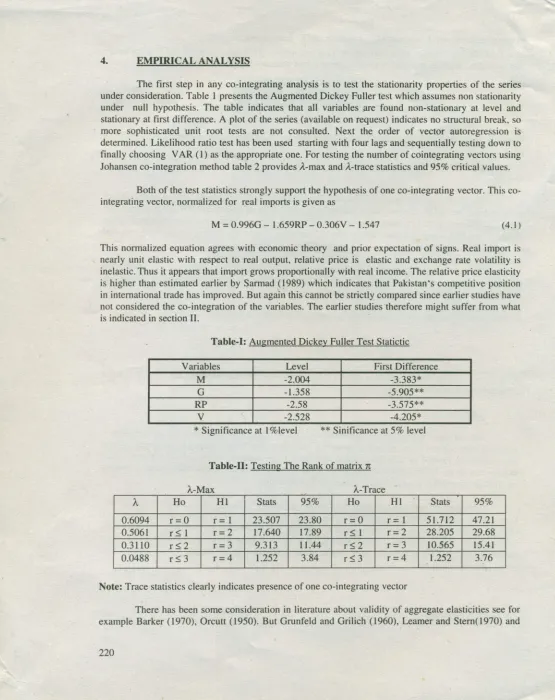
E M P I R I C A L ANALYSIS

The first step in any co-integrating analysis is to test the stationarity properties of the series under consideration. Table

SRQPONMLKJIHGFEDCBA

Ipresents the Augmented Dickey Fuller test which assumes non stationarity under null hypothesis. The table indicates that all variables .are found non-stationary at level and stationary at first difference. A plot of the series (available on request) indicates no structural break, so

more sophisticated unit root tests are not consulted. Next the order of vector autoregression is

determined. Likelihood ratio test has been used starting with four lags and sequentially testing down to finally choosing V AR (I) as the appropriate one. For testing the number of cointegrating vectors using Johansen co-integration method table 2 provides A-max and A-trace statistics and 95% critical values.

Both of the test statistics strongly support the hypothesis of one co-integrating vector. This co-integrating vector, normalized for real imports is given as

M = 0.996G - 1.659RP - 0.306V - 1.547 (4.1 )

[image:5.579.8.563.33.733.2]

This normalized equation agrees with economic theory and prior expectation of signs. Real import is nearly unit elastic with respect to real output, relative price is elastic and exchange rate volatility is inelastic. Thus it appears that import grows proportionally with real income. The relative price elasticity is higher than estimated earlier by Sarmad (1989) which indicates that Pakistan's competitive position in international trade has improved. But again this cannot be strictly compared since earlier studies have not considered the co-integration of the variables. The earlier studies therefore might suffer from what is indicated in section II.

Table-I: Augmented Dickey Fuller Test Statictic

Variables Level First Difference

M -2.004 -3.383*

G -1.358 -5.905**

RP -2.58 -3.575**

V -2.528 -4.205*

* Significance at I %Ievel ** Sinificance at 5% level

Table-II: Testing The Rank of matrix 1 t

--A Ho HI Stats 95% Ho HI Stats 95%

0.6094 r= 0 r = 1 23.507 23.80 r=O r= 1 51.712 47.21

0.5061 r::; 1 r= 2 17.640 17.89 r::; 1 r= 2 28.205 29.68

0.3110 r< 2 r= 3 9.313 11.44 r::; 2 r= 3 10.565 15.41

0.0488 r::; 3 r=4 1.252 3.84 r::; 3 r=4 1.252 3.76

A-Max A-Trace

Note: Trace statistics clearly indicates presence of one co-integrating vector

There has been some consideration in literature about validity of aggregate elasticities see for

Aigner and Goldfeld (1973) provided some evidence that dis-aggregate data may be subject to measurement error than aggreagate data and the predictions obtained from dis-aggregated models may' not be better than those obtained from an aggregate model.

4.1 Impulse response function

To investigate further the relationship between imports and its determinants. another tool is impulse response function. This shows how each endogenous variable responds to shock in other variable. That is the Impulse response function traces the response of the endogenous variable to one standard deviation shock in each variable in the system. This is displayed graphically in figure 1.

Figure 1 trace the response of innovation in each variable on real imports. The highest negative impact over time that is increasing gradually is of real relative prices. While a shock in output and volatility have little effect 'on the equilibrium value of import. A shock in import in previous periods will have its positive effect. which is gradually increasing.

4.2 Variance Decomposition

Another way of characterizing the dynamic behavior of the model is through variance decomposition. This breaks down the variance of the forecast error from each variable into components that can be attributed to each of the endogenous variable. Table III shows the variance decomposition of each variable. The first column indicates forecast horizon. The second column shows percentage of

real imports forecast error variance that can be attributed to real import itself. Similarly

SRQPONMLKJIHGFEDCBA

3 , d , 4 t h and 5t h columns show the percentage of real import forecast variance that can be attributed to real output,

relative prices and exchange rate volatility, respectively.

For example panel (a) shows that the most significant effect on imports is of relative prices that is gradually increasing reaching 38% in tenth year. Output and volatility have relatively smaller. Panel (b) shows that initially imports have some effect on output but its role is gradually decreasing. In the longer horizon relative prices and volatility becoming important for explaining variance in output. Panel (c) shows that after 5 period 38% variance in relative prices is due to import which is slowly decreasing. Panel (d) shows that the variables in the system have little effect of volatility. This confirms our similar observation from the causality test.

Fi

0.3

0.2

0.1

0

-0.1

-0.2

-0.3

~

---_ ---_ ---_ ---_ ---_ ---_ ---_ ---_ ---_ ---_ ---_ ---_ ---_ ---_ ---_ L _ _

1 . " - _ ' \ 4 F i

RQPONMLKJIHGFEDCBA

7 R ! = l T O

--

--

FEDCBA

_{- - - -}

---1 - -

i m p o r t - - - . O u t p u t - - - P r i c e s - - V o l a t i l i t y

I

T a b l e - I I I :

rqponmlkjihgfedcbaZYXWVUTSRQPONMLKJIHGFEDCBA

Decomposition Of Forecast Error Variance

Percentage Of forecast variance explained by shocks in:

SRQPONMLKJIHGFEDCBA

M G

RP

_V

Year Relative Variance In M

1 100.00 0.00 0.00 0.00

2 90.32 0.63 8.35 0.70

3 82.40 0.92 16.12 0.57

4 76.91 1.05 21.52 0.52

5 72.80 1.09 25.53 0.58

1 0 59.13 0.90 37.79 2.18

Year Relative Variance In G

i 9.86 90.14 0.00 0.00

2 3.26 48.92 1.47 46.36

3 1.40 33.73 9.38 55.48

4 0.69 23.00 16.72 59.58

5 0.42 16.82 23.32 59.44

1 0 0.33 5.86 40.99 52.82

Year Relative Variance In RP

1 45.52 0.00 54.48 0.00

2 41.36 1.19 57.45 0.00

3 40.14 1.33 58.32 0.22

4 39.28 1.46 58.97 0.29

5 38.63 1.50 59.54 0.33

1 0 36.06 1.45 62.31 0.18

Year Relative Variance In V

1 2.58 8.08 9.26 80.08

2 4.30 4.35 8.48 82.86

3 4.57 3.92 8.43 83.08

4 4.81 3.59 8.70 82.90

5 4.95 3.45 9.07 82.53

1 0 5.48 3.14 11.61 79.78

5.

CONCLUSIONS

There appears to be a single co-integration vector which asserts that real import is nearly unit elastic

with respect to real outpui, relative price is unit elastic and' exchange rate volatility is inelastic.

Proportional growth of import with output has led some researchers (e.g. Milas (1998) in case of

Greece) to suggest that, to improve balance of trade. output growth should be restricted in some way

for example by increasing taxes. We optimistically suggest not to constrained or hinder output growth.

The elastic relative prices is seen to favor devaluation to reduce imports and improve trade balance.

'Since Pakistan's import mainly consist of items that are conducive to growth in output, devaluation

cannot be recommended. This leaves export promotion as a viable option to improve trade balance.

REFERENCES

l. Aigner, DJ. and Goldfeld, S.M. (1973). Simulation and Aggregation: a reconsideration.

RQPONMLKJIHGFEDCBA

R e v i e w

o f E c o n o m i c s a n d S t a t i s t i c s , 55, 114-118.

2. Akhter, M. and Hilton, R.S. (1984). Effects of exchange rate uncertainty on German and U.S.

trade. Federal Reserve Bank of New York Quarterly Review, Spring, 7-16.

error-correction 'models. R e v i e w o f E c o n o m i c s a n d S t a t i s t i c s , LXXV(4), 700,706.

3. Ariz, A.C. and Shwiff, S.S.( 1998). Does exchange rate volatility affects trade flows in G-7

countries? evidence from Co-integration model. A p p l i e d E c o n o m i c s , 30, 1269-1276.

4. Barker (1970). Aggregation error and estimation of U.K. import demand function. in the

econometric study of United Kingdom. Ed. K. Hilton and D.E. Heathfeld, Macmillan,

London.

5. Chowdhry, A.R. (1993). Does exchange rate volatility depress trade flows? evidence from error

-correction models. R e v i e w o f E c o n o m i c s a n d S t a t i s t i c s , LXXV( 4),700-706.

6. Dickey, D.A. and Fuller, W.A. (1979). Distribution of the estimators for autoregressive time

series with a unit root. J o u r n a l O f A m e r i c a n S t a t i s t i c a l A s s o c i a t i o n , 74, 427-433.

7. Dickey, D.A. and Fuller, W.A. (1981). Likelihood Ratio Statistics for autoregressive time series

with a unit root. E c o n o m e t r i c a , 49, 1057-1072.

8. Enders, W. (1995). Applied Econometric Time Series. John Wiley, New York.

9. Engle, R.F an GrangerC.WT. (l98i). 'Co-integration -an correction: representation,

estimation and testing. E c o n o m e t r i c a , 55, 251-276.

10. Fuller, W.A. (1985). Non-stationary autoregressive time series in EJ. Hannan et al Handbook of

Statistics 5.

It. Gafar, J.S. (1988). The determinants of import demand in Trinidad and Tobago. A p p l i e d

E c o n o m i c s , 20, 303-313.

12. Granger, C.WJ and Newbold, P. (1974). Spurious regression in Econometrics. J o u r n a l O f

Economtrics, 2, 111-120.

13. Grunfeld, Y and Griliches, Z.(1960). Is aggregation necessarily bad? R e v i e w O f E c o n o m i c s a n d

S t a t i s t i c s , 42, 1-13.

14. Johansen, S. (1988). Statistical Analysis of co-integrating vectors. J o u r n a l O f E c o n o m i c

D y n a m i c s A n d C o n t r o l , 12,231-254.

15. Johansen, S. (1991). Estimation and hypothesis testing of Co-interation vectors in Gaussian

autoregressive models. E c o n o m e t r i c a , 59, 1551-1580.

16. Johansen, Sand Juselius, K.(J 990). Maximum Likelihood estimation and inference in

Co-integration with application to demand for money. O x f o r d B u l l e t i n O f E c o n o m i c s a n d

S t a t i s t i c s , 52,169 ..210.

17. Khan, M.S. and Ross.

SRQPONMLKJIHGFEDCBA

K . Z . (1979). The functional form 0' the aggregate import demand