Periodogram and Ensemble Empirica
Mode Decomposition Analysis of
Electromyography Processing
S. Elouaham
ESSI, National School of
Applied Sciences, Ibn Zohr University Agadir, MoroccoR. Latif
ESSI, National School of
Applied Sciences, Ibn Zohr University Agadir, MoroccoA.
Dliou
ESSI, National School of
Applied Sciences, Ibn Zohr University Agadir, MoroccoF. M. R. Maoulainine
Team of Child, Health and Development, CHU, Faculty of Medicine, Cadi Ayyad University,
Marrakech, Morocco
ABSTRACT
This work investigates the application of the Ensemble Empirical Mode Decomposition (EEMD) and the time-frequency techniques for treatment of the electromyography (EMG) signal. The EMG signals are usually corrupted by artifacts that hide useful information then the extraction of high-resolution EMG signals from recordings contaminated with back ground noise becomes an important problem. The Ensemble Empirical Mode Decomposition (EEMD) is used for overcoming the noise problem. Due to the non-stationary of EMG signals, the analysis of this signal with the time-frequency techniques is inevitable. These time-time-frequency techniques are capable to reveal and extract the multicomponents of the EMG signal. The different time-frequency techniques used in this work are parametric techniques such as Periodogram, Capon and Lagunas and non-parametric such as Smoothed Pseudo Wigner-Ville and Hilbert Spectrum. These time-frequency techniques were applied to a normal and abnormal EMG signals, these signals were taken from patients with neuropathy and myopathy pathologies respectively. The results show that The Periodogram technique presents a powerful tool for analyzing the EMG signals. This study shows that the combination of the EEMD and the Periodogram techniques are a good issue in the biomedical field.
Keywords:
EEMD, Time-frequency, Periodogram, Capon, Lagunas, SPWV, Hilbert spectrum, EMG.1.
INTRODUCTION
Electromyography (EMG) is an experimental technique concerned with the development, recording and analysis of myoelectric signals. Myoelectric signals are formed by physiological variations in the state of muscle fiber membranes. The measurements of the electrical activity of muscles are recorded with the placement of small metal discs, called electrodes applied to the skin’s surface. The objective of our study is to detect muscle fatigue from the electromyogram EMG signal analysis [1]. In clinical EMG is consist of the waveforms called the Motor Unit Action Potentials (MUAPs) which are recorded by using a needle electrode at slight voluntary contraction [2-6]. The shape, size
and frequency of the MUAPs are the factors of classifying the normal and abnormal of EMG signals. The detection of MUAPs reflects the electrical activity of a single anatomical Motor Unit. It represents the compound action potential of those muscle fibers within the recording range of the electrode. The own EMG signal is a condition for an appropriate interpretation. Due to the multiplicity of recording electrodes and their contact zone tiny electrode-skin, contamination of noise appears as a problem even more difficult. This noise perturbs the good visualization of information. For overcome this problem various methods have been used to denoising the biomedical signals such as Wavelet Transform (WT) and Empirical mode decomposition (EMD). These techniques have some drawbacks at level the reconstruction of the original signal. The drawbacks of WT are their non-adaptive basis due to the selection process of the basis function that is controlled by the signal components that are relatively large in a frequency band [7-9]. The EMD is a recently developed method used for analyzing the nonlinear and non-stationary signal. This technique represents signals as sums of simpler components with amplitude and frequency modulated parameters, the major problem of the original EMD is the appearance of mode-mixing [10-12]. To overcome these problems the noise- assisted data analysis method, called the Ensemble Empirical Mode Decomposition (EEMD) is proposed by Wu and Huang [12].
Periodogram (PE), Capon (CA) and Lagunas (LAG) and non parametric time-frequency techniques, Smoothed Pseudo Wigner-Ville (SPWV) and Hilbert Spectrum (HS) are applied to analyze EMG signals. These time-frequency methods are applied over modulated signals for giving the robust technique that eliminates the cross-terms and presents high resolution on the time-frequency plan. The EMG signals used are normal and abnormal, collected from the patients with neuropathy and myopathy [29]. The parametric and non-parametric time– frequency techniques were used to evaluate exercise-induced changes in the biological EMG signal and also to study the type of MUAPs recruited in specific phases of the movement.
In the following study, the theoretical of Ensemble Empirical Mode Decomposition (EEMD) and the parametric and non-parametric time-frequency techniques are presented in section 2. In the section 3, we will give the used signals and we will present the main results the section 4 and 5. The conclusion for this work is given in Section 6.
2.
TEORETICAL TECHNIQUES
2.1
EEMD
The EMD was recently proposed by Huang et al. as a tool to adaptively decompose a signal into a collection of AM–FM components. The EMD method has no mathematical foundations and analytical expressions for the theoretical study. The various works has successfully used the EMD to real data in several fields such as biomedical, study of phenomena climate, seismology or acoustics [10-12]. These studies show satisfaction and matching condition used in non-stationary signal processing. EMD decomposes adaptively non-stationary signal into a sum of functions oscillatory band-limited d(t) called Intrinsic Mode Functions IMFJ(t). By
definition these functions IMFJ(t) oscillate around zero and
can express the signal x(t) by the expression:
( ) ( ) ( ) 1
k
x t dj t r t j
(1)
Where r(t) is the residue of low frequency.
By definition, each IMFJ(t) must satisfy two conditions:
a) The number of zero crossings and the number of extreme signal must be equal throughout the analyzed signal,
b) At any point, the average of the envelopes defined by local extreme of the signal must be 0.
The higher order IMFJ(t) correspond to low oscillation
components, while lower-order IMFJ(t) represents fast
oscillations. For different decomposed signals the number of IMFJ(t) is variable. It also depends on the spectral content of
the signal. The Rilling study presents the technical aspects of the EMD implementation and makes the five-step algorithm given by the following:
a) Extract the extreme of the signal x(t),
b) Deduce an upper envelope emax (t) (resp. lower emin (t)) by
interpolation of the maxima (resp minima),
c) Define a local average m(t) as the sum of the half-envelopes:
m t
( )
(
e
max
( )
t
e
min
( )) / 2
t
(2)d) Deduce a local detail; dJ(t)=IMFJ(t) by the expression:
d
j
( )
t
x t
( )
m t
( )
(3)e) The iteration is given by the expression (1).
The first IMF contains the terms of higher frequencies and contains the following terms of decreasing frequency up to forward only a residue of low frequency. The ensemble EMD method has been offered for overcome mode mixing problem existing in EMD technique. The EEMD technique allows giving all solution that gives the true IMF by repeating the decomposition processes. The procedure of the EEMD method is given as follow [12]:
Step 1: Add white noise with predefined noise amplitude to the signal to be analyzed.
Step 2: Use the EMD method to decompose the newly generated signal.
Step 3: Repeat the above signal decomposition with different white noise, in which the amplitude of the added white noise is fixed.
Step 4: Calculate the ensemble means of the decomposition results as final results.
The signal x(k), is decomposed into a finite number of intrinsic mode functions (IMFs) and a residue.
( )
1
in
x k
c
r
i
(4)Where n represents the number of the IMFs, ci is the ith IMF that is the ensemble mean of the corresponding IMF
obtained from all of decomposition processes and r
is the mean of the residues from all of decomposition processes.
2.2
TIME-FREQUENCY ANALYSIS
The time-frequency technique is a tool to treatment non-stationary signal, which used time and frequency simultaneously to represent the non-stationary signal.
2.2.1
Parametric techniques
The parametric time-frequency techniques used in this work are the Capon, Lagunas and the Periodogram.
2.2.1.1
Capon distribution
The estimator of minimum variance called Capon estimator (CA) does not impose a model on the signal. At each frequency f, this method seeks a matched filter whose response is 1 for the frequency f and 0 everywhere else [14-15].
( , ) ( , ) ( , ) 1
1
. .
H
CA n f a n f R a n fx
H
Zf Rx n Zf
Where:
- CA n f
,
is the output power of the filter Capon, excitedby the discrete signal x(n) sampled at the period te,
- a n f
,
a0,...,a p
is the impulse response of thefilter at frequency n,
-
T
Rx n E x n x n is the autocorrelation matrix of
crossed x(n) of dimension
p1 * p1 ,- x n
x n p ,...,x n
is the signal at time n,- ZfH
1,e2i ft e,...,e2i ft p e
is the steering vector,- (p+1) is the number of filter coefficient and the exponent H for conjugate transpose and the superscript T for transpose.
2.2.1.2
Periodogram technique
The Periodogram (PE) is the derivate of the Capon (CA) technique. The spectral estimator of this method is defined by the following equation [10]:
PE n f( , )ZHf .R Zx. f / ((p+1) )2 (6)
The two previous techniques defined by the equations 5 and 6 can be applied sliding windows. There is no theoretical criterion for choosing the filter order and duration of the window [17]. The parametric techniques depend on the signal so that the frequency response has a different shape and then different properties according to the signal characteristics. The choice of the window is more crucial to the time-frequency resolution. CA and PE estimator usually has a better frequency resolution. Both techniques are well suited to signals containing some strong spectral components such as ECG and EMG biomedical signals.
2.2.1.3
Lagunas technique:
CA f( ) is homogeneous to power but not to a spectral
density function since the area under the estimated function does not represent the total power of the analyzed signal. Lagunas [16, 17] proposed a method to derive the spectral density from the minimum variance power. The time– frequency distribution LAG (t, f), of x(t) can be obtained as:
1 ( , )
2 H Zf Rx Zf
LAG t f te
H
Z Rx Z
f f
(7)
The x(t) be a discrete and non stationary signal sampled at frequency fe = 1/te.
2.2.2
Non-parametric time frequency techniques
2.2.2.1
Smoothed Pseudo Wigner-Ville (SPWV)
The majority of the non parametric time-frequency representations are represented by the cohen class [20-28]. This class includes inter alias the Smoothed Pseudo Wigner-Ville [20-24]. Among the large number of existing non parametric time-frequency representations some authors have proposed using the SPWV. To avoid the covering of
frequential components in the time-frequency representation of Wigner-ville, in this study we use in the place of the real signal x t( ) the analytical signalxa( )t . This signal is defined
by the expression:
xa( )t x t( )iH x t{ ( )} (8)
Where i2 =-1, x t( )is the signal with real values and H x t{ ( )}
it’s the Hilbert transform. The spectrum Fa( )k of the
analytical signal xa( )t is given by:
2 ( ) 0 / 2
( ) (0) 0, / 2
0 / 2
X k if k N F ka X if k N
if N k N
(9)
Where X(k) is the Fourier transform of the original signal x(t) and N is the number of points.
The distribution of Wigner-Ville associated to a signalx t( )
, of finished energy, is the function Wxa depending of the
temporal (t) and frequential (f) parameters. This distribution is given by the following expression [20-24]:
( , ) .* 2
2 2
i f Wxa t f xatxat e d
(10)
Where * a
x indicates the complex conjugate ofxa( )t .
The transform called the Smoothed Pseudo Wigner-Ville is implanted in this study to attenuate the interference terms presented between the inner components figured in Wigner-Ville image. These terms decrease the visibility of the time-frequency image [20-24]. The SPWV use two smoothing windows h(t) and g(t). These smoothing windows are introduced into the Wigner-Ville distribution definition in order to allow a separate control of interference either in time (g) or in frequency (h). The expression of this representation is defined by [20-24]:
2
2 * ( , )
2 2 2
a
i f SPWVx t f h g t u x ua x ua e d du
(11)
The great disadvantage of the SPWV technique is the presence of cross-terms. These cross-terms can hide the information of signal and also analyze the time–frequency image becomes difficult.
2.2.2.2
Hilbert transform
y t( ) P x( )d t
(12)
Where P is the Cauchy principal value,
The Hilbert transform is capable of identifying the local properties of the signal x(t). The analytic signal z(t) of x(t) can be obtained by coupling the signal x(t) and its Hilbert transform y(t):
z t( )x t( )iy t( )a t e( ) i( )t (13)
Where:
- 2 2
( ) ( ) ( )
a t x t y t is the instantaneous amplitude of
( )
x t
,- ( ) arctan ( ) ( ) y t t
x t
is the instantaneous phase of
x t
( )
.The controversial instantaneous frequency ω(t) is defined as the time derivative of the instantaneous phase
( )
t
as follows:( )t d ( )t dt
(14)
The equation (13) gives both the amplitude and the frequency of each component as functions of time. It also enables us to represent the amplitude and the instantaneous frequency as functions of time in a three-dimensional plot, in which the amplitude can be contoured on the frequency-time plan.
3.
Analysis of EMG signals using the
EEMD
[image:4.595.318.574.71.203.2]The electromyogram (EMG) signal is a common clinical test used to assess function of muscles and the nerves that control them. The EMG studies are used to help in the diagnosis and management of disorders such as the muscular dystrophies and neuropathies. Nerve conduction studies that measure how well and how fast the nerves conduct impulses are often performed in conjunction with EMG studies [3-5]. The figures 1(a), 2 (a) and 3 (a) show three examples of EMG signals: for the first signal 1 (a): a 44 year old man without history of neuromuscular disease; for the second signal 2 (a): a 57 year old man with myopathy due to longstanding history of polymyositis, treated effectively with steroids and low-dose methotrexate and for the third signal: a 62 year old man with chronic low back pain and neuropathy due to a right L5 radiculopathy; and The data were recorded at 50 KHz and then down sampled to 4 KHz. The EMG signals are often interfered by noises. These artifacts strongly influence the utility of recorded EMG signals. The EEMD technique allows us to remove the artifact existing in the analyzed signal by eliminating the first IMFs. The figure 1 presents the results obtained by using EEMD on normal EMG signal the noise added is 11 db.
Fig 1: Normal EMG signal (a), noised signal (b) and the reconstruction without noise (c)
[image:4.595.318.573.292.428.2]
The figure 2 presents the results obtained by using EEMD on signal of the patient with myopathy, we also add noise of 11 db.
Fig 2: Abnormal (myopathy) EMG signal (a), noised signal (b) and the reconstruction without noise (c)
The figure 3 presents the results obtained by using EEMD on signal of the patient with neuropathy. We also add noise of 11 db.
Fig 3: Abnormal (neuropathy) EMG signal (a), noised signal (b) and the reconstruction without noise (c)
[image:4.595.318.579.515.666.2]reconstruction signals of the normal EMG and abnormal such as myopathy and neuropathy have largely restored the original shape and clearly eliminates noises of these signals. The EEMD is a powerful technique that eliminates the noises without losing the useful information aid giving the good diagnostic.
4.
PERFORMANCE THE
TIME-FREQUENCY TECHNIQUES
The aim of this study is the choice of the time-frequency technique suitable for assessing localized muscle fatigue during dynamic contractions. The time-frequency techniques are applied in this section on modulated signals for comparing between images; the obtained result allows giving the technique appropriate. The variance factor is also more important tool for choice the technique robust.
4.1
Time-frequency images
The figure 4 compares the results obtained from four distinct parametric and non parametric time–frequency techniques PE,
[image:5.595.71.532.298.513.2]CA, LAG and SPWV. The figure fig.4a present the modulated signal used. The Fourier transform spectrum presented in figure 4b show the evolution of frequency content from 50 to 165; the Fourier transform cannot give information about number of the components frequency and his change on time. The figure 4c presented by PE technique gives a good localization of the two high frequency components that are separated clearly, this result is more clearly than the results obtained by CA, LAG and SPWV techniques in figure 4d, 4e and 4f respectively. The figure 4f shows the presence of strong cross-terms and the resolution decrease such that the two high frequency components cannot be discriminated.
Fig 4: Modulated signal (a), Fourier spectrum (b), Periodogram (c), Capon (d), Lagunas (e), SPWV (f)
4.2
Variance factor
The time-frequency techniques used in this study are applied to a monocomponent signal to find the most performance technique. The monocomponent signal used is given by the following equation:
x t( )aej( )t (14)
The instantaneous frequency (IF) is given by the following equation:
1 / 0 2
f d dt f t
(15)
Where a=1, fo=0.05fs, = 0.4fs, ( )t is the analytic signal
phase and fs = 1/T is the sampling frequency.
The bias (B) and the variance (V) of the estimate present the most important factors that decide the quality of estimation. These two notions can be defined by the following
expressions:
( ) ( )
B fi t fi t
(16)
2
( ) ( ( ))
V f i t f i t
(17)
Were:
( ) fi t
= f ti( )- f i( )t
Where f ti( ) and fi( )t
are the instantaneous frequency and instantaneous frequency estimate respectively. The signal length used in the time-frequency techniques is N=256 samples and the total signal duration is 1 s. The sampling frequency was fs=2 NHz. Using different Signal-to-Noise
Ratio (SNR), gaussian white noise samples are added to the signal. The figure 8 shows the performance of the PE, CA, LA and SPWV time-frequency techniques applied to a linear FM a
d b
c
f
signal with 256 points. According to the results obtained, the Periodogram time-frequency technique has a minimal variance for all SNR's. The low minimum variance can indicate the performance of the time-frequency techniques.
Fig 5: Performance of Variance of various techniques PE, CA, LAG and SPWV of a linear FM signal with length
N = 256 samples
The results obtained by the time-frequency images and the variance factors show the effectiveness the PE time-frequency
technique.
5.
RESULTS
The aim of this work is to conclude which is the best time-frequency technique among the different techniques chosen in this paper. This conclusion will be made from the results obtained by the application of the different time-frequency techniques over the EMG signals. The quality of the technique will be deduced according to the cross-terms level and the resolution.
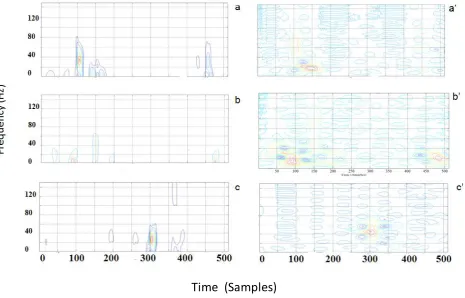
In this section, the time-frequency techniques PE, SPWV and HS are applied to the normal and abnormal EMG signals (figures 1 (a), 2 (a) and 3 (a) respectively). The Figure 6 shows the corresponding time-frequency images obtained by PE and SPWV and the figure 7 displays the time–frequency spectrum obtained by executing Hilbert transform to the IMFs obtained by EEMD.
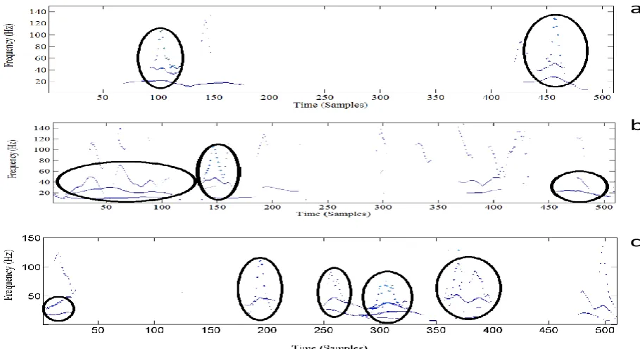
[image:6.595.70.536.319.617.2]Fig 7: Time–frequency spectrum based on EEMD. a) Healthy, b) Myopathy and c) Neuropathy
In EMG signals, the detection of MUAPs is important because it allows providing the good information about the neuromuscular system. This information is obtained through the morphology and firing time of MUAPs. The time-frequency techniques allow revealing the MUAPs time-frequency components of the normal and abnormal EMG signals. The time-frequency images of the PE technique (fig.6 (a, b and c)) of the normal, myopathy and neuropathy EMG signals respectively (figures 1a, 2a and 3a) give a good localization of the EMG MUAPs in the frequency plan. The time-frequency images of the SPWV technique (fig. 6 (a’, b’, and c’)) give a localization of the MUAPs terms with the presence cross-terms. These cross-terms make the visualization of the MUAPs activity extremely difficult. The images obtained by Hilbert spectral technique (fig.7 (a, b and c)) contain all the significant energy components with interference-terms. We can note that the parametric time-frequency images show to be more efficient in identifying the MUAPs terms of the normal and abnormal EMG signal than the non parametric ones. We can deduce some important features of the normal and abnormal EMG signals by the interpretation of the images obtained by PE technique: for the normal subject the MUAPs are well localized appearing both in time and frequency very clearly with high amplitude. The frequency range selected was between 0 and 82 Hz in time (25 to 180 and 450 to 475). For the myopathy; the MUAPs appear both in time and frequency very clearly with low amplitude. The frequency range selected was between 0 and 65 Hz in time (25 to 200 and 450 to 500). On the other hand, for the neuropathy the energy appearing very clearly with high amplitude. The frequency range selected was between 0 and 60 Hz in time (180 to 400). The PE technique can reveal information about the MUAPs components that can be useful for the identification of the presence of the EMG signal. The high
resolution given by PE is very clearly figured in the time-frequency plan compared to the others time-time-frequency techniques, SPWV and Hilbert spectrum.
6.
CONCLUSION
In this paper, the EEMD and some interesting time-frequency techniques (PE, SPWV and HS) were applied to analyze a normal and abnormal (myopathy and neuropathy) EMG signals. As a first step of the work, the EEMD results obtained show the high effectiveness of this technique for the elimination of the EMG signal artifacts which are due to different noises. In the second step, the time-frequency analysis results show that the PE technique can provide a clear visualization of MUAP activity. The results obtained by SPWV and HS are more difficult to interpret because they were affected by the cross terms, these cross terms make the identification of the MUAPs extremely difficult in the time-frequency plan. We conclude that the PE technique present a high resolution of detecting of the MUAPs activity as compared to the others time-frequency techniques used in this paper. The combination of the EEMD and PE techniques can be a good issue in analyzing the EMG signals.
7.
References
[1] Christodoulou CI., Pattichis CS. 1999. Unsupervided pattern recognition for the classification of EMG signals. IEEE Trans Biomed Eng, Vol. 46 issue 2, pp.169–78.
[2] Sbasi A., Yilmaz M., Ozcalik H. 2006. Classification of EMG signals using wavelet neural network, Journal of Neuroscience Methods, Vol. 156, Issues 1–2, pp. 360– 367.
[3] Hussain MS., and Mohd-Yasin F. 2006. Techniques of EMG signal analysis: detection, processing, classification and applications. Biol. Proced. Online 8(1), pp.11-35.
[4] Bonato P., Boissy P., Della Croce U., Roy SH. 2002. Changes in the surface EMG signal and the
a
biomechanics of motion during a repetitive lifting task. IEEE Trans Neural Syst Rehabil Eng, Vol. 10, pp. 38– 47.
[5] Bonato P., Roy SH., Knaflitz M., De Luca CJ. 2001. Time–frequency parameters of the surface myoelectric signal for assessing muscle fatigue during cyclic dynamic contractions. IEEE Trans Biomed Eng Vol.48,Issue 7, pp. 745-753
[6] Kimura J. 2001. Electrodiagnosis in Diseases of Nerve and Muscle: Principles and Practice, 3rd Edition. New York, Oxford University Press.
[7] Alfaouri M., Daqrouq K. 2008. ECG signal denoising by wavelet transform thresholding, American Journal of Applied Sciences, Vol. 5, pp. 276–281.
[8] Sayadi O., Shamsollahi M. 2006. ECG denoising with adaptive bionic wavelet transform, in: 28th Annual International Conference of the IEEE Engineering in Medicine and Biology Society, EMBS ’06, pp. 6597– 6600.
[9] Kopsinis Y., McLaughlin S. 2009. Development of EMD-based denoising methods inspired by wavelet thresholding, IEEE Transactions on Signal Processing 57, pp.1351–1362.
[10]Elouaham S., Latif R., Dliou A., Maoulainine F. M. R., Laaboubi M. 2012. Analysis of biomedical signals by the empirical mode decomposition and parametric time-frequency techniques, International Symposium on security and safety of Complex Systems, May 25-26, Agadir, Morocco.
[11]Blanco-velasco M., Weng B., Kenneth E. 2008. ECG signal denoising and baseline wander correction based on the empirical mode decomposition, computers in biology and medicine, Vol. 38, pp.1-13.
[12] Wang T., Zhang M., Yu Q., Zhang H. 2012. Comparing the applications of EMD and EEMD on time–frequency analysis of seismic signal, Journal of Applied Geophysics, Vol. 83, pp.29–34.
[13]Michele G., Sello S., Carboncini MC., Rossi B., Strambi S. 2003. Cross-correlation time–frequency analysis for multiple EMG signals in Parkinson’s disease: a wavelet approach,Medical Engineering & Physics, Vol, 25, Issue 5, pp. 361-369.
[14]Özgen, M.T. 2003. Extension of the Capon’s spectral estimator to time–frequency analysis and to the analysis of polynomial-phase signals, Signal Process, Vol. 83, n.3, pp. 575–592.
[15]Elouaham S., Latif R., Dliou A., Aassif E., Nassiri B. 2011. Analyse et comparaison d’un signal ECG normal et bruité par la technique temps-frequence parametrique de capon, Conference Mediterranéene sur l’Ingenierie Sure des Systemes Complexes MISC’11, Mai 27-28, Agadir, Maroc.
[16] Lagunas M.A., Santamaria M.E., A. Gasull, A. Moreno. 1986. Maximum likelihood filters in spectral estimation problems, journal Signal Processing, Vol. 10 Issue 1, pp. 19 – 34.
[17]Castanié F. 2006. Spectral Analysis Parametric and Non-Parametric Digital Methods, (ISTE Ltd, USA, pp. 175-211.
[18]Goncalves P., Auger F., Flandrin P. 1995. Time-frequency toolbox.
[19]Flandrin, P., Martin, N., Basseville M. 1992. méthodes temps-fréquence (Trait. Signal 9).
[20]Latif R., Aassif E., Maze G., Moudden A., Faiz B. 1999. Determination of the group and phase velocities from time-frequency representation of Wigner-Ville", Journal of Non Destructive Testing & Evaluation International, Vol. 32 n.7, pp. 415-422.
[21]Latif R., Aassif E., Maze G., Decultot D., Moudden A., Faiz B. 2000. Analysis of the circumferential acoustic waves backscattered by a tube using the time-frequency representation of wigner-ville, Journal of Measurement Science and Technology, Vol. 11, n. 1, pp. 83-88.
[22]Latif R., Aassif E., Moudden A., Faiz B., Maze G. 2006. The experimental signal of a multilayer structure analysis by the time-frequency and spectral methods, NDT&E International, Vol. 39, n. 5, pp. 349-355.
[23]Latif R., Aassif E., Moudden A., Faiz B. 2003. High resolution time-frequency analysis of an acoustic signal backscattered by a cylindrical shell using a Modified Wigner-Ville representation, Meas. Sci. Technol.14, pp. 1063-1067.
[24]Latif R., Laaboubi M., Aassif E., Maze G. 2009, Détermination de l’épaisseur d’un tube élastique à partir de l’analyse temps-fréquence de Wigner-Ville, Journal Acta-Acustica, Vol. 95, n. 5, pp. 843-848.
[25]Pachori R.B., Sircar P. 2007. A new technique to reduce cross terms in the Wigner distribution, Digital Signal Processing, Vol. 17, pp.466–474.
[26]Dliou A., Latif R., Laaboubi M., Maoulainine F. M. R. 2012. Arrhythmia ECG Signal Analysis using Non Parametric Time-Frequency Techniques, International Journal of Computer Applications (0975 – 8887), Vol. 41, No.4,
[27]Dliou A., Latif R., Laaboubi M., Maoulainine F. M. R. 2012. Abnormal ECG Signal Analysis using Non Parametric Time-Frequency Techniques, Arabien Journal of Science Engineering (Accepted).
[28] Choi H., Williams, W. 1989. Improved time-frequency representation of multicomponent signals using exponential kernels”, IEEE Trans. on Acoustics, Speech and Signal Processing, vol. 37, pp. 862-871.