Formulation of a Preconditioned Algorithm for the Conjugate Gradient Squared Method in Accordance with Its Logical Structure

(1)

http://dx.doi.org/10.4236/am.2015.68131

How to cite this paper: Itoh, S. and Sugihara, M. (2015) Formulation of a Preconditioned Algorithm for the Conjugate Gra-dient Squared Method in Accordance with Its Logical Structure. Applied Mathematics, 6, 1389-1406.

http://dx.doi.org/10.4236/am.2015.68131

Formulation of a Preconditioned Algorithm

for the Conjugate Gradient Squared Method

in Accordance with Its Logical Structure

Shoji Itoh

1

, Masaaki Sugihara

2

1_{Division of Science, School of Science and Engineering, Tokyo Denki University, Saitama, Japan}

2_{Department of Physics and Mathematics, College of Science and Engineering, Aoyama Gakuin University,}

Kanagawa, Japan Email: [email protected]

Received 22 June 2015; accepted 27 July 2015; published 30 July 2015

This work is licensed under the Creative Commons Attribution-NonCommercial International License (CC BY-NC).

http://creativecommons.org/licenses/by-nc/4.0/

Abstract

In this paper, we propose an improved preconditioned algorithm for the conjugate gradient squared method (improved PCGS) for the solution of linear equations. Further, the logical struc-tures underlying the formation of this preconditioned algorithm are demonstrated via a number of theorems. This improved PCGS algorithm retains some mathematical properties that are asso-ciated with the CGS derivation from the bi-conjugate gradient method under a non-preconditioned system. A series of numerical comparisons with the conventional PCGS illustrate the enhanced ef-fectiveness of our improved scheme with a variety of preconditioners. This logical structure un-derlying the formation of the improved PCGS brings a spillover effect from various bi-Lanczos-type algorithms with minimal residual operations, because these algorithms were constructed by adopt-ing the idea behind the derivation of CGS. These bi-Lanczos-type algorithms are very important because they are often adopted to solve the systems of linear equations that arise from large-scale numerical simulations.

Keywords

Linear Systems, Krylov Subspace Method, Bi-Lanczos Algorithm, Preconditioned System, PCGS

1. Introduction

(2)

1390

Ax=b (1) where A is a large, sparse coefficient matrix of size n n× , x is the solution vector, and b is the right-hand side (RHS) vector.

The conjugate gradient squared (CGS) method is a way to solve (1) [1]. The CGS method is a type of bi- Lanczos algorithm that belongs to the class of Krylov subspace methods.

Bi-Lanczos-type algorithms are derived from the bi-conjugate gradient (BiCG) method [2] [3], which as-sumes the existence of a dual system

T # #

.

A x =b (2) Characteristically, the coefficient matrix of (2) is the transpose of A. In this paper, we term (2) a “shadow system”.

Bi-Lanczos-type algorithms have the advantage of requiring less memory than Arnoldi-type algorithms, another class of Krylov subspace methods.

The CGS method is derived from BiCG. Furthermore, various bi-Lanczos-type algorithms, such as BiCGStab [4], GPBiCG [5] and so on, have been constructed by adopting the idea behind the derivation of CGS. These bi-Lanczos-type algorithms are very important because they are often adopted to solve systems in the form of (1) that arise from large-scale numerical simulations.

Many iterative methods, including bi-Lanczos algorithms, are often applied together with some precondition-ing operation. Such algorithms are called preconditioned algorithms; for example, preconditioned CGS (PCGS). The application of preconditioning operations to iterative methods effectively enhances their performance. In-deed, the effects attributable to different preconditioning operations are greater than those produced by different iterative methods [6]. However, if a preconditioned algorithm is poorly designed, there may be no beneficial ef-fect from the preconditioning operation.

Consequently, PCGS holds an important position within the Krylov subspace methods. In this paper, we iden-tify a mathematical issue with the conventional PCGS algorithm, and propose an improved PCGS1. This im-proved PCGS algorithm is derived rationally in accordance with its logical structure.

In this paper, preconditionedalgorithm and preconditionedsystem refer to solving algorithms described with some preconditioning operator M (or preconditioner, preconditioning matrix) and the system converted by the operator based on M, respectively. These terms never indicate thealgorithmforthepreconditioningoperation itself, such as “incomplete LU decomposition”, “approximate inverse”, and so on. For example, for a precondi-tioned system, the original linear system (1) becomes

,

=

Ax



b

(3)

1 1 1

, , ,

L R R L

A=M−AM− x=M x b=M−b (4) under the preconditioner M =M M_L _R

(

M ≈A

)

. Here, the matrix and the vector in the preconditioned system are denoted by the tilde

( )

 . However, the conversions in (3) and (4) are not implemented; rather, we construct the preconditioned algorithm that is equivalent to solving (3).

This paper is organized as follows. Section 2 provides an overview of the derivation of the CGS method and the properties of two scalar coefficients (α_k and β_k). This forms an important part of our argument for the preconditioned BiCG and PCGS algorithms in the next section. Section 3 introduces the PCGS algorithm. An issue with the conventional PCGS algorithm is identified, and an improved algorithm is proposed. In Section 4, we present some numerical results to demonstrate the effect of the improved PCGS algorithm with a variety of preconditioners. As a consequence, the effectiveness of the improved algorithm is clearly established. Finally, our conclusions are presented in Section 5.

2. Derivation of the CGS Method and Preconditioned Algorithm of the BiCG Method

In this section, we derive the CGS method from the BiCG method, and introduce the preconditioned BiCG

algo-1

This improved PCGS was proposed in Ref. [7] from a viewpoint of deriving process’s logic, but this manuscript demonstrates some ma-thematical theorems underlying the deriving process’s logic. Further, numerical results using ILU(0) preconditioner only are shown in Ref.

(3)

1391

rithm.

2.1. Structure of the BiCG Method

BiCG [2] [3] is an iterative method for linear systems in which the coefficient matrix A is nonsymmetric. The algorithm proceeds as follows:

Algorithm 1. BiCG method:

0

x is an initial guess, r₀ = −b Ax₀, set β−₁=0,

(

#

)

0, 0 ≠0

r r , e.g., # 0 = 0,

r r

For k=0,1, 2,, until convergence, Do:

# # #

1 1, 1 1,

k = +k βk− k− k = k +βk− k−

p r p p r p

(

)

(

)

#

# ,

, ,

k k

k

k A k

α

= r r

p p (5)

1 ,

k+ = k+αk k

x x p

# # T #

1 , 1 ,

k+ = −k αkA k k+ = k −αkA k

r r p r r p

(

)

(

)

# 1 1 #

, , ,

k k

k

k k

β

+ +

= r r

r r (6)

End Do

BiCG implements the following Theorems.

( )

1

( )

1 1

( )

( )

# T #

0,

k = k A

p P r (13)

where r₀ = −b Ax₀ is the initial residual vector and # # T # 0 = −A 0

r b x is the initial shadow residual vector. However, in practice, #

0

r is set in such a way as to satisfy the conditions

(

#

)

0, 0 ≠0

r r .

( )

T

, =

u v u v denotes the inner product between vectors u and v. In this paper, we set #

0 = 0

r r to satisfy the conditions

(

#

)

0, 0 ≠0

r r

2

(4)

1392

( )

)

0 0 0 0

, , , ,

k k = k A k A = k A

)

0 0 0 0

, , , ,

k A k = k A A k A = A k A

p p P r P r r P r (17)

and the following theorem can be applied.

Theorem 3 (Sonneveld [1]) TheCGScoefficients α_k and β_k areequivalent to these coefficients in BiCG under certain transformation and substitution operations based on the bi-orthogonality and bi-conjugacy condi-tions.

Proof. We apply

( )

CGS 2 CGS 2

0, 0

k ≡ k A k ≡ k A

r R r p P r (18)

to (16) and (17). Then,

(

)

(

)

(

( )

)

(

)

(

)

# # 2 # CGS

0 0 0

BiCG CGS

# # 2 # CGS

0 0 0

, , ,

,

, , ,

k k k k

k k

k k k k

A

A A A A

α

= r r = r r = r r ≡

α

p p p r r p

R

P (19)

(

)

(

)

(

( )

)

(

)

(

)

# # 2 # CGS

1 1 0 1 0 0 1

BiCG CGS

# # 2 # CGS

0 0 0

, , ,

.

, , ,

k k k k

k k

k k k k

A A

β

= r+ r+ = r + r = r r+ ≡

β

r r r r r r

R

R (20)

( ) ( )

( )

2 2

1 1

2 2 2

1 1 1 1

2 .

k k k k

k k k k k k

λ

β

λ

β

λ

β

λ

− −

− − − −

= +

= + +

P R P

R P R P (22)

q P R r . □ Thus, we have derived the CGS method4.

3_{In this paper, if we specifically distinguish this algorithm, we write} BiCG

k

α and BiCG

k

β .

4_{In this paper, we use the superscript “CGS” alongside} k

(5)

1393

Algorithm 2. CGS method:

0

x is an initial guess, r₀= −b Ax₀, set CGS 1 0,

β− =

(

#

)

0, 0 ≠0

r r , e.g., # 0 = 0,

r r

CGS CGS 1 1,

k = k +βk− k−

u r q

(

)

CGS CGS CGS CGS

1 1 1 1 ,

k = k+βk− k− +βk− k−

p u q p

(

)

(

)

# CGS 0 CGS

# CGS 0

, , ,

k k

k

A

α

= r r

(

)

# CGS

0 1

CGS

# CGS 0

, , ,

k

β

= r r+

r r

End Do

The following Proposition 5 and Corollary 1 are given as a supplementary explanation for Algorithm 2. These are almost trivial, but are comparatively important in the next section’s discussion.

Proposition 5 Thereexistthefollowingrelations:

CGS 0 = 0,

r r (23)

CGS # # 0 = 0,

r r (24)

where CGS 0

r is the initial residual vector at

k

=

0

in the iterative part of CGS, CGS # 0

r is the initial shadow re-sidual vector in CGS, r₀ is the initial residual vector, and #

0

r is the initial shadow residual vector. Proof. Equation (23) follows because (18) for

k

=

0

gives CGS 2

( )

0 = 0 A 0= 0

r R r r . Here, R₀

( )

A =I by (7), and I denotes the identity matrix.

) (

CGS # CGS

)

0 0 0 0 0

, , , , .

k k = k A k A = k A ≡ k

r r R r R r r R r r r

This equation shows that the inner product of the CGS on the right is obtained from the inner product of the BiCG on the left. Therefore, #

0

r that composes the polynomial

( )

T # 0

k A r

R to express the shadow residual vector of the BiCG is the same as CGS #

0

r in CGS. Hereafter, CGS #

0

r can be represented by # 0

r , to the extent that neither can be distinguished. □ Corollary 1. Thereexiststhefollowingrelation:

CGS CGS 0 = 0 = 0,

p r r

where CGS 0

p is the probing direction vector in CGS, CGS 0

r is the initial residual vector at

k

=

0

in the itera-tive part of CGS, and r₀ is the initial residual vector.

2.3. Derivation of Preconditioned BiCG Algorithm

In this subsection, the preconditioned BiCG algorithm is derived from the non-preconditioned BiCG method (Algorithm 1). First, some basic aspects of the BiCG method under a preconditioned system are expressed, and a standard preconditioned BiCG algorithm is given.

(6)

1394

,

Ax=b (25) we obtain a “BiCG method under a preconditioned system” (Algorithm 3). We denote this as “PBiCG”.

In this paper, matrices and vectors under the preconditioned system are denoted with “”, such as A, p_k5. The coefficients α_k, β_k are specified by PBiCG

k

α , PBiCG

k

β .

Algorithm 3. BiCG method under the preconditioned system:

0

x is an initial guess, r₀ = −b Ax₀, set PBiCG

1 0

β₋ = ,

(

#

)

0, 0 ≠0

r r , e.g., # 0 = 0,

r r

PBiCG # # PBiCG #

1 1, 1 1,

k = +k βk− k− k = k +βk− k−

p r p p r p

(

)

(

)

# PBiCG

# ,

, ,

k k k

k A k

α = r r

p p

  

  (26)

PBiCG

1 ,

k+ = k+αk k

x x p

PBiCG # # PBiCG T #

1 , 1 ,

k+ = −k αk A k k+ = k −αk A k

r r p r r  p

(

)

(

)

# 1 1 PBiCG

# ,

, ,

k k

k

k k

β

+ +

= r r

r r

 

  (27)

End Do

We now state Theorem 6 and Theorem 7, which are clearly derived from Theorem 1 and Theorem 2, respec-tively.

Theorem 6. Under the preconditioned system, there are recurrence relations that define the degree k of the residual polynomial R_k

( )

λ

 andprobingdirectionpolynomial P_k

( )

λ

 6.Theseare

( )

0 1, 0 1,

− P−

λ

 (30)

where λ is the variation under the preconditioned system, and PBiCG

k

α , PBiCG

k

β in these relations are based on (26) and (27).

Using the polynomials of Theorem 6, the residual vectors of the preconditioned linear system (25) and the shadow residual vectors of the following preconditioned shadow system:

T # #

A x =b (31) can be represented as

( )

0,

k =Rk A

r  r (32)

( )

# T #

0,

k =Rk A

r  r (33)

respectively. The probing direction vectors are given by

( )

0,

k =P Ak

p  r (34)

5_{If we wish to emphasize different methods, a superscript is applied to the relevant vectors to denote the method, such as} PBiCG

k

p , BiCG

k



p .

(7)

1395

( )

# T #

0,

k =P Ak

p  r (35)

respectively. Under the preconditioned system, # 0

r is set in such a way as to satisfy the conditions

(

#

)

0, 0 ≠0

r r . In this paper, we set #

0

, 0 bi-conjugacy conditions under the preconditioned system .

i A j = i≠ j

p p (37)

Next, we derive the standard PBiCG algorithm. Here, the preconditioned linear system (25) and its shadow system (31) are formed as follows:

(

1 1

)

(

)

1

,

L R R L

M− AM− M x =M−b (38)

(

T T T

)(

T #

)

T #

.

R L L R

M− A M− M x =M− b (39)

Definition 1. OnthesubjectofthePBiCGalgorithm, thesolutionvectorisdenotedas PBiCG

k

x .Furthermore, theresidualvectorsofthelinearsystemandshadowsystemofthePBiCGalgorithmarewrittenas PBiCG

k

r and

PBiCG #

k

r , respectively, andtheirprobingdirectionvectorsare PBiCG

k

p and PBiCG #

k

p , respectively.

Using this notation, each vector of the BiCG under the preconditioned system given by Algorithm 3 is con-verted as below:

1 PBiCG_, # T PBiCG #_, PBiCG_, # T PBiCG #_.

k ML k k MR k k MR k k ML k

− −

= = = =

r r r r p p p p (40)

Substituting the elements of (40) into (36) and (37), we have

(

#_,

) (

T PBiCG #_, 1 PBiCG

) (

PBiCG #_, 1 PBiCG

)

_,

i j MR i ML j i M j

− − −

, , , .

i A j ML i ML AMR MR j i A j

− −

= =

p p p p p p (42)

Consequently, (26) and (27) become

(

)

(

)

(

)

# PBiCG # 1 PBiCG PBiCG

PBiCG # PBiCG #

, ,

,

k k k k

k k k k k M A A α −

= r r = r r

p p

  

  (43)

(

)

(

)

(

)

# PBiCG # 1 PBiCG

1 1 1 1

PBiCG

# PBiCG # 1 PBiCG

, ,

.

, ,

k k k k

k

k k k k

M M

β

− + + + + −

= r r = r r

r r r r

 

  (44)

Before the iterative step, we give the following Definition 2.

Definition 2. Forsomepreconditionedalgorithms, theinitialresidualvectorofthelinearsystemiswrittenas

P 0

r andtheinitialshadowresidualvectoroftheshadowsystemiswrittenas P # 0

r beforetheiterativestep. We adopt the following preconditioning conversion after (40).

1 P # T P # 0 ML 0 , 0 MR 0 .

− −

= =

r r r r (45)

Consequently, we can derive the following standard PBiCG algorithm [9] [10].

Algorithm 4. Standard preconditioned BiCG algorithm:

0

x is an initial guess, P

0 = −A 0,

r b x set PBiCG

1 0

(8)

1396

(

#

) (

P # 1 P

)

0, 0 0 ,M 0 0

−

= ≠

r r r r , e.g., P # 1 P

0 M 0,

−

=

r r

PBiCG 1 PBiCG PBiCG PBiCG 1 1 ,

k M k βk k

−

− −

= +

p r p

PBiCG # T PBiCG # PBiCG PBiCG #

1 1 ,

k M k βk k

−

− −

= +

p r p

(

)

(

)

PBiCG # 1 PBiCG PBiCG

PBiCG # PBiCG ,

, ,

k k

k

k k

M A

α

−

= r r

p p (46)

PBiCG PBiCG PBiCG PBiCG

1 ,

k+ = k +αk k

x x p

PBiCG PBiCG PBiCG PBiCG

1 ,

k+ = k −αk A k

r r p (47)

PBiCG # PBiCG # PBiCG T PBiCG #

1 ,

k+ = k −αk A k

r r p (48)

(

)

(

)

PBiCG # 1 PBiCG

1 1

PBiCG

PBiCG # 1 PBiCG ,

= ,

,

k k

k

k k

M M

β

−

+ +

−

r r

r r (49)

End Do

Algorithm 4 satisfies PBiCG P 0 = 0

r r and PBiCG # P #

0 = 0

r r when

k

=

0

in the iterative part. Remark 2. Becauseweapplya preconditioningconversionsuch as PBiCG

k =MR k

x x intheiterationofthe BiCGmethodunderthepreconditionedsystem (Algorithm 3), PBiCG

0 = 0

x x when

k

=

0

intheiteration of Al-gorithm 4. Further, the initial solution to Algorithm 3 is technically x₀, but this is actually calculated by multiplying M_R bytheinitialsolution x₀.

In this section, we have shown that α_k in BiCG is equivalent to α_k in CGS using (19), and that β_k in BiCG is equivalent to β_k in CGS using (20). In the next section, we propose an improved PCGS algorithm by applying this result to the preconditioned system.

3. Improved PCGS Algorithm

In this section, we first explain the derivation of PCGS, and present the conventional PCGS algorithm. We iden-tify an issue with this conventional PCGS algorithm, and propose an improved PCGS that overcomes this issue.

[image:8.595.170.456.541.704.2]

3.1. Derivation of PCGS Algorithm

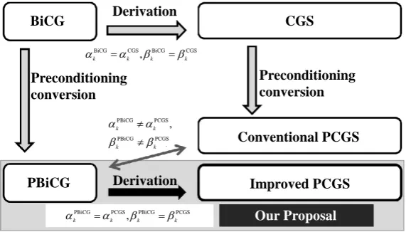
Figure 1 illustrates the logical structure of the solving methods and preconditioned algorithms discussed in this paper.

CGS BiCG

PBiCG

Conventional PCGS

Improved PCGS Derivation

Preconditioning conversion Preconditioning

conversion

Derivation

BiCG CGS BiCG CGS

,

k k k k

α =α β =β

PBiCG PCGS PBiCG PCGS

,

k k k k

α =α β =β Our Proposal

PBiCG PCGS

,

k k

α α

β β

≠ ≠

(9)

1397

Typically, PCGS algorithms are derived via a “CGS method under a preconditioned system” (Algorithm 5). Algorithm 5 is derived by applying the CGS method (Algorithm 2) to the preconditioned linear system (25). In this section, the vectors and α_k, β_k are PCGS elements, except for those before the iteration (Definition 2). If we wish to emphasize different methods, we apply a superscript to the relevant vectors, such as PCGS

k

α ,

PCGS

k

β , PCGS

k

p , CGS

k

p .

Algorithm 5. CGS method under the preconditioned system:

0

x is an initial guess, r₀ = −b Ax₀, set PCGS

1 0

β₋ = ,

(

#

)

0, 0 ≠0

r r , e.g., # 0 = 0

r r ,

PCGS 1 1,

k = +k βk− k−

u r q

(

)

PCGS PCGS

1 1 1 1 ,

p u q p

(

)

(

)

# 0 0 PCGS # 0 , , , k k A

α = r r

r p      PCGS , k = k−αk A k

q u p

(

)

PCGS

1 ,

k+ = k+

α

k k+ k

x x u q

(

)

PCGS

1 ,

k+ = −k

α

k A k + k

r r  u q

(

)

(

)

# 0 1 PCGS # 0 , , , k k k

β

+

= r r

r r

   

End Do

The conventional PCGS algorithm (Algorithm 6) is derived via the CGS method, as shown inFigure 1, but this algorithm does not reflect the logic of subsection 2.2 in its preconditioning conversion. In contrast, our pro-posed improved PCGS algorithm (Algorithm 7) directly applies the derivation from BiCG to CGS to the PBiCG algorithm, thus maintaining the logic from subsection 2.2.

3.2. Conventional PCGS and Its Issue

The conventional PCGS algorithm is adopted in many documents and numerical libraries [4] [9] [11]. It is de-rived by applying the following preconditioning conversion to Algorithm 5:

1 1 1 1

# T # 1 1 1

0 0

, , , ,

, , , .

L R k R k L k L k

L k L k k L k k L k

A M AM M M M

M M M M

− − − −

− − −

= = = =

x x b b r r

r r p p u u q q

 _  _

    (50)

This gives the following Algorithm 6 (“Conventional PCGS” in Figure 1).

Algorithm 6. Conventional PCGS algorithm:

0

x is an initial guess, r₀ = −b Ax₀,

(

#

)

0, 0 ≠0

r r , e.g., # 0 = 0,

r r set β−₁=0,

1 1,

k = +k βk− k−

u r q

(

)

1 1 1 1 ,

p u q p

(

)

(

)

# 0 # 1 0 , , , k k k AM

)

(

)

# 0 1 # 0 , , , k k k

β

= r r+

r r (52)

End Do

This PCGS algorithm was described in [4], which proposed the BiCGStab method, and has been employed as a standard approach as affairs stand now.

This version of PCGS seems to be a compliant algorithm on the surface, because the operation

(

#

)

0, k

r r in (51) and (52) does not include the preconditioning operator M−1 under the conversions 1

k ML k −

=

r r and

# T # 0 =ML 0

r r from (50). However, if we apply # T # 0 =ML 0

r r from (50) to the preconditioning conversion of the shadow residual vector in the BiCG method, we obtain

# T #_.

k =ML k

r r (53)

This is different to the conversion given by (40), and we cannot obtain equivalent coefficients to PBiCG

k

α ,

PBiCG

k

β in (43) and (44) using (53).

3.3. Derivation of the CGS Method from PBiCG

In this subsection, we present an improved PCGS algorithm (“Improved PCGS” in Figure 1). We formulate this algorithm by applying the CGS derivation process to the BiCG method directly under the preconditioned system (PBiCG, Algorithm 3).

The polynomials (32)-(35) of the residual vectors and the probing direction vectors in PBiCG are substituted for the numerators and denominators of PBiCG

k

α and PBiCG

k

)

0 0 0 0

, , , ,

k k = Rk A Rk A = Rk A

)

0 0 0 0

, , ,

k A k = P Ak AP Ak = APk A

p p  r   r r   r (55)

and apply the following Theorem 8.

Theorem 8. The PCGS coefficients α_k and β_k are equivalent to these coefficients in PBiCG under certain transformationandsubstitution operationsbasedon thebi-orthogonality andbi-conjugacy conditions underthepreconditionedsystem.

Proof. We apply

( )

CGS 2 CGS 2

0, 0

k ≡Rk A k ≡Pk A

r  r p  r (56)

to (54) and (55). Then,

(

)

(

)

(

)

BiCG # BiCG # CGS 0

PBiCG PCGS

BiCG # BiCG # CGS 0

, ,

,

, ,

k k k

k k

k A k A k

α = r r = r r ≡α

p p r p

   

 

    (57)

(

)

(

)

(

)

BiCG # BiCG # CGS

1 1 0 1

PBiCG PCGS

BiCG # BiCG # CGS 0

, ,

.

, ,

k k k

k k

k k k

β

= r+ r+ = r r+ ≡

β

r r r r

   

    (58)

□ The PCGS method is derived from PBiCG using Theorem 9.

(11)

solu-1399 tion vector CGS

k

x isderivedfromarecurrencerelationbasedon CGS CGS

k = −A k

r b x .

Proof. The coefficients α_k and β_k in PBiCG and PCGS were derived in Theorem 8. The recurrence rela-tions in (29) and (30) for PBiCG are squared to give:

( )

(

( )

)

2

( )

( ) ( )

( )

2 2 2 2 2

1 1 1 1 2 1 1 1 1 1 ,

k k k k k k k k k k

)

2

( )

( ) ( )

( )

2 2 2 2

1 1 2 1 1 1 1 .

k k k k k k k k k k

 (60)

Further, we can apply rkCGS≡Rk2

( )

A r ₀, pCGSk ≡Pk2

( )

A r₀ from (56), and substitute

( ) ( )

CGS

0

k ≡P A Rk k A

u   r ,

( ) ( )

CGS

1 0

k ≡P A Rk k+ A

q   r. □ The following Proposition 10 and Corollary 2 are given as a supplementary explanation under the precondi-tioned system.

Proposition 10. Thereexistthefollowingrelations:

CGS 0 = 0,

r r (61)

CGS # # 0 = 0,

r r (62)

where r₀CGS is the initial residual vector at

k

=

0

in the iterative part of PCGS, r₀CGS # is the initial shadow residual vector in PCGS, r₀ is the initial residual vector, and r₀# is the initial shadow residual vector.

Proof. Equation (61) follows because (56) for

k

=

0

gives r0CGS=R02

( )

A r0=r0. Here, R0

( )

A =I by (28). Equation (62) is derived as follows. Applying (56) to (54), we obtain

(

BiCG # BiCG

)

(

( )

T #

( )

)

(

# 2

( )

)

(

CGS # CGS

)

0 0 0 0 0

, , , , .

k k = Rk A Rk A = Rk A ≡ k

       

r r r r r r r r

This equation shows that the inner product of the PCGS on the right is obtained from the inner product of the PBiCG on the left. Therefore, #

0

r that composes the polynomial Rk

( )

A T r0# to express the shadow residual vector of the PBiCG is the same as CGS #

0

r in PCGS. Hereafter, CGS #

0

r can be represented by # 0

r , to the extent that neither can be distinguished. □ Corollary 2. Thereexiststhefollowingrelation:

CGS CGS 0 = 0 = 0,

p r r

where CGS 0

p is the probing direction vector in PCGS, CGS 0

r is the initial residual vector at

k

=

0

in the itera-tive part of PCGS, and r₀ is the initial residual vector.

The CGS preconditioning conversion given by CGS

k

r , CGS

k

p , and # 0

r is subjected to the same treatment as the BiCG preconditioning conversion of r_k, p_k, in (40) and (45). Further, P #

0

r is the same as # 0

r . Then,

(

)

(

)

(

)(

)

(

)

# CGS T # 1 PCGS # 1 PCGS

0 0 0

PCGS

# 1 PCGS

# CGS T # 1 1 PCGS

0 0 0 , , , , , , ,

k R L k k

k

k R L R R k

M M M

M A

A M M AM M

α

− − −

−

− − −

= r r = r r = r r

r p

r p r p

  

  (63)

(

)

(

)

(

)

(

)

# C T # 1 PCGS # 1 PCGS

0 1 0 1 0 1

P

# C T # 1 PCGS # 1 PCGS

0 0 0

, , ,

.

, , ,

GS

k R L k k

CGS

k _GS

k R L k k

M M M

β

− − − + + + − − − =   = =  

r r r r r r

(64)

As a consequence, the following improved PCGS algorithm is derived7.

Algorithm 7. Improved preconditioned CGS algorithm:

0

x is an initial guess, r₀ = −b Ax₀,

(

#

)

0, 0 ≠0

r r , e.g., # 1 0 M 0,

−

=

r r set β−₁=0, For k=0,1, 2,, until convergence, Do:

1

1 1,

k M k βk k

−

− −

= +

u r q

7_{We apply the superscript “PCGS” to} k

(12)

1400

(

)

1 1 1 1 ,

p u q p

(

)

(

)

# 1

0

# 1

0 ,

, ,

k

M

M A

α

−

= r r

r p

1 _,

(

)

# 1

0 1

# 1

0 ,

, ,

k

M M

β

− + −

= r r

r r

End Do

Algorithm 7 can also be derived by applying the following preconditioning conversion to Algorithm 5. Here, we treat the preconditioning conversions of u_k and q_k the same as the conversion of p_k.

1 1 1 1

# T #

0 0

, , , ,

, , , .

L R k R k L k L k

R k R k k R k k R k

A M AM M M M

M M M M

− − − −

−

= = = =

x x b b r r

r r p p u u q q

 _  _

   

The number of preconditioning operations in the iterative part of Algorithm 7 is the same as that in Algorithm 6.

4. Numerical Experiments

In this section, we compare the conventional and improved PCGS algorithms numerically.

The test problems were generated by building real unsymmetric matrices corresponding to linear systems taken from the Tim Davis collection [12] and the Matrix Market [13]. The RHS vector b of (1) was generated by setting all elements of the exact solution vector x_exact to 1.0, and substituting this into (1). The solution al-gorithm was implemented using the sequential mode of the Lis numerical computation library (version 1.1.2 [14]) in double-precision, with the compiler options registered in the Lis “Makefile”. Furthermore, we set the in-itial solution to x₀ =0, and considered the algorithm to have converged when 12

2

2 1.0 10

k

−

≤ ×

r b (where

k

r is the residual vector in the algorithm, and k is the iteration number). The maximum number of iterations was set to the size of the coefficient matrix.

The numerical experiments were executed on a DELL Precision T7400 (Intel Xeon E5420, 2.5 GHz CPU, 16 GB RAM) running the Cent OS (kernel 2.6.18) and the Intel icc 10.1 compiler.

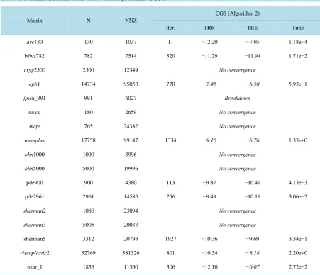
The results using the non-preconditioned CGS are listed inTable 1.

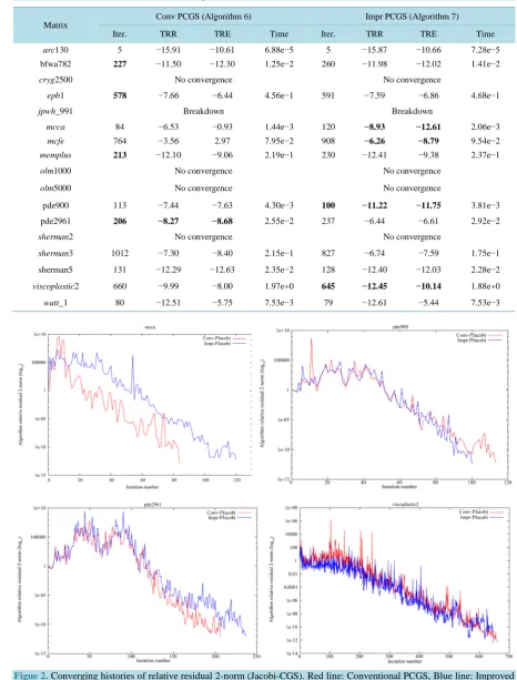
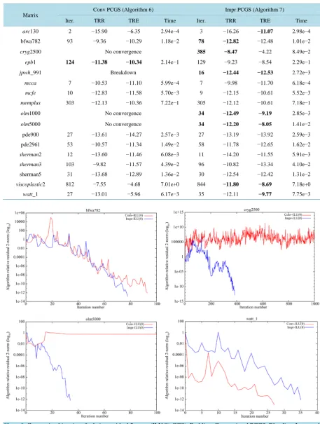
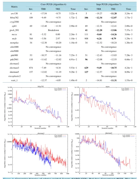
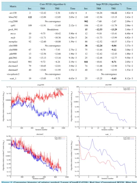
The results given by the conventional PCGS and the improved PCGS are listed in Tables 2-5. Each table adopts a different preconditioner in Lis [14]: “(Point-)Jacobi”, “ILU(0)”8, “SAINV”, and “Crout ILU”. In these tables, significant advantages of one algorithm over the other are emphasized by bold font9. Additionally, ma-trix names given in italic font inTable 1encounter some difficulties. The evolution of the convergence for each preconditioner is shown inFigures 2-5. In this paper, we do not compare the computational speed of these pre-conditioners.

In many cases, the results given by the improved PCGS are better than those from the conventional algorithm. We should pay particular attention to the results from matrices “mcca”, “mcfe” and “watt_1”. In these cases, it appears that the conventional PCGS converges faster with any preconditioner, but the TRE values are worse than those from the improved algorithm. The iteration number for the conventional PCGS is not emphasized by bold font in these instances. The consequences of this anomaly are worth investigating further, possibly by ana-lyzing them under PBiCG. This will be the subject of future work.

8_{Values of “zero” for ILU(0) indicates the fill-in level, that is, “no fill-in”.}

9_{Because the principal argument presented in this paper concerns the structure of the algorithm for PCGS based on an improved}

(13)

[image:13.595.85.537.93.481.2]

1401

Table 1.Numerical results for a veriety of test problems (CGS).

Matrix N NNZ

CGS (Algorithm 2)

Iter. TRR TRE Time

arc130 130 1037 11 −12.20 −7.05 1.18e−4

bfwa782 782 7514 320 −11.29 −11.94 1.71e−2

cryg2500 2500 12349 No convergence

epb1 14734 95053 770 −7.45 −6.50 5.93e−1

jpwh_991 991 6027 Breakdown

mcca 180 2659 No convergence

mcfe 765 24382 No convergence

memplus 17758 99147 1334 −9.16 −6.76 1.33e+0

olm1000 1000 3996 No convergence

olm5000 5000 19996 No convergence

pde900 900 4380 113 −9.87 −10.49 4.13e−3

pde2961 2961 14585 256 −9.49 −10.19 3.06e−2

sherman2 1080 23094 No convergence

sherman3 5005 20033 No convergence

sherman5 3312 20793 1927 −10.36 −9.69 3.34e−1

viscoplastic2 32769 381326 801 −10.34 −8.18 2.20e+0

watt_1 1856 11360 306 −12.10 −6.07 2.72e−2

In this table, “N” is the problem size and “NNZ” is the number of nonzero elements. The items in each column are, from left to right, the number of iterations required to converge (denoted “Iter.”), the true relative residual log10 2-norm (denoted by “TRR”, calculated as b−Axˆk ₂ b₂, where

ˆk

x is the numerical solution), the true relative error log10 2-norm (denoted by “TRE”, calculated from the numerical solution and the exact solution,

that is, xˆ_k−x_exact₂ x_exact₂), and, as a reference, the CPU time (denoted “Time” [s]). Several matrix names are represented in italicfont. These describe certain situations, such as “Breakdown”, “No convergence”, and insufficient accuracy on “TRR” or “TRE”.

5. Conclusions

In this paper, we have developed an improved PCGS algorithm by applying the procedure for deriving CGS to the BiCG method under a preconditioned system, and we also have presented some mathematical theorems un-derlying the deriving process’s logic. The improved PCGS does not increase the number of preconditioning op-erations in the iterative part of the algorithm. Our numerical results established that solutions obtained with the proposed algorithm are superior to those from the conventional algorithm for a variety of preconditioners.

However, the improved algorithm may still break down during the iterative procedure. This is an artefact of certain characteristics of the non-preconditioned BiCG and CGS methods, mainly the operations based on the bi-orthogonality and bi-conjugacy conditions. Nevertheless, this improved logic can be applied to other bi- Lanczos-based algorithms with minimal residual operations.

In future work, we will analyze the mechanism of the conventional and improved PCGS algorithms, and con-sider other variations of this algorithm. Furthermore, we will concon-sider other settings of the initial shadow resi-dual vector r0#, except for

# 0 = 0

r r to ensure that

(

#

)

0, 0 ≠0

(14)

[image:14.595.74.541.95.709.2]

1402

Table 2. Numerical results for a veriety of test problems (Jacobi-CGS).

Matrix

Conv PCGS (Algorithm 6) Impr PCGS (Algorithm 7)

Iter. TRR TRE Time Iter. TRR TRE Time

arc130 5 −15.91 −10.61 6.88e−5 5 −15.87 −10.66 7.28e−5 bfwa782 227 −11.50 −12.30 1.25e−2 260 −11.98 −12.02 1.41e−2

cryg2500 No convergence No convergence

epb1 578 −7.66 −6.44 4.56e−1 591 −7.59 −6.86 4.68e−1

jpwh_991 Breakdown Breakdown

mcca 84 −6.53 −0.93 1.44e−3 120 −8.93 −12.61 2.06e−3

mcfe 764 −3.56 2.97 7.95e−2 908 −6.26 −8.79 9.54e−2

memplus 213 −12.10 −9.06 2.19e−1 230 −12.41 −9.38 2.37e−1

olm1000 No convergence No convergence

pde900 113 −7.44 −7.63 4.30e−3 100 −11.22 −11.75 3.81e−3

pde2961 206 −8.27 −8.68 2.55e−2 237 −6.44 −6.61 2.92e−2

sherman2 No convergence No convergence

sherman3 1012 −7.30 −8.40 2.15e−1 827 −6.74 −7.59 1.75e−1

sherman5 131 −12.29 −12.63 2.35e−2 128 −12.40 −12.03 2.28e−2

viscoplastic2 660 −9.99 −8.00 1.97e+0 645 −12.45 −10.14 1.88e+0

watt_1 80 −12.51 −5.75 7.53e−3 79 −12.61 −5.44 7.53e−3

(15)

[image:15.595.81.539.96.702.2]

1403

Table 3.Numerical results for a veriety of test problems (ILU(0)-CGS).

Matrix

arc130 2 −15.90 −6.35 2.94e−4 3 −16.26 −11.07 2.98e−4 bfwa782 93 −9.36 −10.29 1.18e−2 78 −12.82 −12.48 1.01e−2

cryg2500 No convergence 385 −8.47 −4.22 8.49e−2

epb1 124 −11.38 −10.34 2.14e−1 129 −9.23 −8.54 2.29e−1

jpwh_991 Breakdown 16 −12.44 −12.53 2.72e−3

mcca 7 −10.53 −11.10 5.99e−4 7 −9.98 −11.70 6.18e−4

mcfe 10 −12.83 −11.58 5.70e−3 9 −12.15 −10.61 5.52e−3

memplus 303 −12.13 −10.36 7.22e−1 305 −12.12 −10.61 7.18e−1

olm1000 No convergence 34 −12.49 −9.19 2.85e−3

pde900 27 −13.61 −14.27 2.57e−3 27 −13.19 −13.92 2.59e−3 pde2961 53 −10.57 −11.34 1.49e−2 58 −11.78 −12.65 1.62e−2

sherman2 12 −13.60 −11.46 6.08e−3 11 −14.20 −11.55 5.91e−3

sherman3 103 −9.82 −11.57 4.39e−2 96 −10.82 −13.34 4.10e−2

sherman5 31 −13.68 −12.89 1.36e−2 30 −12.54 −12.42 1.31e−2

viscoplastic2 812 −7.55 −4.68 7.01e+0 844 −11.80 −8.69 7.18e+0

watt_1 27 −13.01 −5.96 6.17e−3 35 −12.11 −9.77 7.75e−3

(16)

[image:16.595.76.541.95.703.2]

1404

Table 4. Numerical results for a veriety of test problems (SAINV-CGS).

Matrix

arc130 4 −17.54 −8.75 3.22e−4 5 −19.27 −11.20 3.24e−4 bfwa782 109 −9.49 −9.75 1.72e−2 106 −12.34 −12.07 1.73e−2

cryg2500 No convergence No convergence

epb1 69 −12.40 −11.91 2.90e+0 69 −12.31 −12.41 2.89e+0

jpwh_991 Breakdown 41 −12.20 −13.06 7.37e−3

mcca 81 −5.32 0.00 2.26e−3 111 −8.60 −14.26 3.04e−3

mcfe 764 −3.56 2.97 1.10e−1 908 −6.26 −8.79 1.29e−1

memplus 34 −12.30 −10.20 1.18e+0 34 −12.32 −10.24 1.20e+0

pde900 53 −10.37 −11.16 7.25e−3 51 −12.43 −13.03 7.28e−3 pde2961 110 −11.62 −12.02 6.91e−2 96 −12.08 −12.55 6.66e−2

sherman2 No convergence No convergence

sherman3 874 −7.49 −8.34 5.53e−1 629 −9.49 −10.75 4.24e−1 sherman5 157 −12.02 −11.19 9.20e−2 127 −12.57 −12.30 8.09e−2

viscoplastic2 No convergence No convergence

watt_1 1 −12.37 −4.05 1.49e+0 2 −14.81 −11.31 1.53e+0

[image:16.595.87.541.100.695.2]

(17)

[image:17.595.81.539.95.705.2]

1405

Table 5. Numerical results for a veriety of test problems (CroutILU-CGS).

Matrix Conv PCGS (Algorithm 6) Impr PCGS (Algorithm 7)

arc130 2 −12.42 −2.34 1.63e−4 4 −16.26 −11.12 1.82e−4 bfwa782 122 −12.09 −12.05 2.03e−2 149 −12.56 −13.15 2.42e−2

cryg2500 No convergence 902 −7.60 −2.67 2.09e−1

epb1 109 −11.91 −11.69 2.12e−1 106 −12.10 −11.79 2.06e−1

jpwh_991 Breakdown 15 −12.53 −13.29 3.46e−3

mcca 10 −9.75 −10.42 5.90e−4 12 −9.10 −15.41 6.40e−4

mcfe 23 −11.71 −10.36 6.24e−3 26 −11.73 −13.99 6.82e−3

memplus 92 −12.60 −10.00 1.59e−1 88 −12.52 −10.57 1.53e−1

olm5000 67 −9.70 −7.93 2.75e−2 75 −11.64 −9.12 3.06e−2 pde900 13 −12.56 −12.66 1.96e−3 12 −12.42 −12.43 1.88e−3 pde2961 24 −13.13 −13.16 9.18e−3 25 −12.48 −12.77 9.50e−3

sherman2 901 −9.72 −6.24 2.19e−1 841 −10.61 −8.71 2.05e−1

sherman3 79 −10.65 −12.01 3.94e−2 74 −11.68 −13.90 3.73e−2

sherman5 40 −13.04 −11.95 1.53e−2 40 −13.30 −12.93 1.53e−2

viscoplastic2 No convergence No convergence

watt_1 19 −13.05 −5.75 6.63e−3 25 −15.25 −9.43 8.12e−3

[image:17.595.86.540.104.695.2]

(18)

1406

Acknowledgements

This work is partially supported by a Grant-in-Aid for Scientific Research (C) No. 25390145 from MEXT, Ja-pan.

References

[1] Sonneveld, P. (1989) CGS, A Fast Lanczos-Type Solver for Nonsymmetric Linear Systems. SIAM Journal on Scienti- fic and Statistical Computing, 10, 36-52.http://dx.doi.org/10.1137/0910004

[2] Fletcher, R. (1976) Conjugate Gradient Methods for Indefinite Systems. In: Watson, G., Ed., Numerical Analysis Dun-dee 1975, Lecture Notes in Mathematics, Vol. 506, Springer-Verlag, Berlin,New York, 73-89.

[3] Lanczos, C. (1952) Solution of Systems of Linear Equations by Minimized Iterations. Journal of Research of the Na-tional Bureau of Standards, 49, 33-53.http://dx.doi.org/10.6028/jres.049.006

[4] Van der Vorst, H.A. (1992) Bi-CGSTAB: A Fast and Smoothly Converging Variant of Bi-CG for the Solution of Nonsymmetric Linear Systems. SIAM Journal on Scientific and Statistical Computing, 13, 631-644.

http://dx.doi.org/10.1137/0913035

[5] Zhang, S.-L. (1997) GPBi-CG: Generalized Product-Type Methods Based on Bi-CG for Solving Nonsymmetric Linear Systems. SIAM Journal on Scientific Computing, 18, 537-551.http://dx.doi.org/10.1137/s1064827592236313

[6] Itoh, S. and Sugihara, M. (2010) Systematic Performance Evaluation of Linear Solvers Using Quality Control Tech-niques. In: Naono, K., Teranishi, K., Cavazos, J. and Suda, R., Eds., Software Automatic Tuning: From Concepts to State-of-the-Art Results, Springer, 135-152.

[7] Itoh, S. and Sugihara, M. (2013) Preconditioned Algorithm of the CGS Method Focusing on Its Deriving Process.

Transactions of the Japan SIAM, 23, 253-286. (in Japanese)

[8] Hestenes, M.R. and Stiefel, E. (1952) Methods of Conjugate Gradients for Solving Linear Systems. Journal of Re-search of the National Bureau of Standards, 49, 409-435.http://dx.doi.org/10.6028/jres.049.044

[9] Barrett, R.,Berry, M., Chan, T.F., Demmel, J., Donato, J., Dongarra, J., et al. (1994) Templates for the Solution of Li-near Systems: Building Blocks for Iterative Methods. SIAM.http://dx.doi.org/10.1137/1.9781611971538

[10] Van der Vorst, H.A. (2003) Iterative Krylov Methods for Large Linear Systems. Cambridge University Press, Cam-bridge.http://dx.doi.org/10.1017/CBO9780511615115

[11] Meurant, G. (2005) Computer Solution of Large Linear Systems. Elsevier,Amsterdam.

[12] Davis, T.A. The University of Florida Sparse Matrix Collection. http://www.cise.ufl.edu/research/sparse/matrices/

[13] Matrix Market Project. http://math.nist.gov/MatrixMarket/