Evaluation of Transition Points between Different Solid Phases in Aqueous Media

http://dx.doi.org/10.4236/jasmi.2014.43012

How to cite this paper:Michałowska-Kaczmarczyk, A.M. and Michałowski, T. (2014) Evaluation of Transition Points be-tween Different Solid Phases in Aqueous Media. Journal of Analytical Sciences, Methods and Instrumentation, 4, 87-94. http://dx.doi.org/10.4236/jasmi.2014.43012

Evaluation of Transition Points between

Different Solid Phases in Aqueous Media

Anna M. Michałowska-Kaczmarczyk1_{, Tadeusz Michałowski}2*

1_{Department of Oncology,The University Hospital in Cracow, Cracow, Poland}

2_{Faculty of Engineering and Chemical Technology, Technical University of Cracow, Cracow, Poland} Email: *_{[email protected]}

Received 3 July 2014; revised 3 August 2014; accepted 10 August 2014

Copyright © 2014 by authors and Scientific Research Publishing Inc.

This work is licensed under the Creative Commons Attribution International License (CC BY).

http://creativecommons.org/licenses/by/4.0/

Abstract

A uniform procedure is suggested for calculation of the pHt value(s) separating equilibrium solid phases in pH scale, at an excess of the precipitating agent. The pHt value, related to pairs of preci-pitates formed from the species Me OH

(

)

_i+ −u i

(

i=1,,p

)

and H Lj j n

+ −

₍

₎

1, ,

j=  q , fulfils the relation n⋅pH+ pL=F, where F is a constant value involving pKso’s for solubility products (Kso’s) of these precipitates, and the equilibrium data, related to the species composing these precipi-tates.

Keywords

Electrolytic Systems, Precipitates, pH-Intervals

1. Introduction

Some species are able to form different solid phases in aqueous media whose composition depends on pH-val- ue of these media. In particular, this was indicated for the systems obtained after introducing the ternary salts such as struvite [1] or dolomite [2] into pure water or aqueous solution of a strong base in presence/absence of CO2, originating e.g. from air. Full physicochemical knowledge was involved in the algorithms used for calcula-tions made according to iterative computer programs related to redox or non-redox, mono- or two-phase systems [3]-[8].

This paper concerns calculations related to two-phase systems, and made with use of Excel spreadsheets. It refers to location of different equilibrium solid phases within defined pH-intervals [9]-[11]. The search of these pH-intervals is based on the simplified calculation procedure. The pH-values separating these intervals are

named as transition

( )

t points, and denoted as pHt.

2. Formulation of the Transition Points

Let the precipitates Mea

(

H Lk

)

_b and Mec

(

H Lm

)

_d, characterized by solubility products:

, Me u a H Lk k n b Kso ab

+ + −

  ⋅  =

    (1)

,

Meu c H Lm n d

m Kso cd

+ + −

  ⋅  =

    (2) be two equilibrium solid phases formed in an aqueous system involving Me+u and L−n

ions, together with the Me OH

( )

_i+ −u i

(

i=1,,p

)

and H Lj j n

+ −

₍

₎

1, ,

j=  q species resulting from hydrolytic phenomena; other (possible) soluble complexes formed between the related species are omitted (not involved) in the related balances. The numbers: a, b, c, d, u, n, k and m in (1) and (2) satisfy the conditions of electro neutrality of the corresponding precipitates:

(

)

au=b n− →k bk=bn−au (3)

(

)

,

cu=d n−m →dm=dn−cu cu+dm=dn (4)

We assume that the Me-species are precipitated with an excess of the L-species; this excess is expressed by the molar concentration:

L 0 H L q j n j j

C• + −

=

 

=

∑

_{ } (5)

If the protonated species do not exist, then L L

n

C• =   − . Applying the stability constants KHj of the

pro-to-complexes, _{H L} j n H _H 1 j _Ln

j Kj

+ − + −

 = ⋅   

     , we denote:

L L L

n

C• =_ − _⋅z (6)

where H 1 L 1 1 H q _i j j

z K +

=

 

= +

∑

_{⋅  } (7)

and H

0 1

K ≡ . Assuming C_L• =const, and the equilibrium solid phases: Mea

(

H Lk

)

b (at pH<pHt1) and

(

)

Mec H Lm d (at pH>pHt1), we state that at transitional pH=pHt1 value, the solubility products: Kso ab, and K_{so cd,} are fulfilled simultaneously, and then from (1) and (2) we get:

( ) ( )

(

) (

)

1 H H

, ,

H bkc dma Ln bc ad bc ad c a

k m so ab so cd

K K − K K

− − −

+ −

  ⋅  ⋅ ⋅ = ⋅

    (8)

Applying in (8) the relations (3) and (4), we have bkc–dma=n bc

(

−ad

)

and then, by turns,

( )

_{( ) ( )}

₍

_{) (}

₎

1 H H

, ,

H n bc ad Ln bc ad Kk bc Km ad Kso ab c Kso cd a

− − − − + −   ⋅  ⋅ ⋅ = ⋅     H H

, , log log

pH pL c pKso ab a pKso cd bc Kk ad Km

n

bc ad

⋅ − ⋅ − ⋅ + ⋅

⋅ + =

− (9)

where pH= −log H_ +1_, pL= −log L_ −n_. Similarly, when the relations: (2) and (10):

1

,

Me u OH u Kso u

+ −

    =

    (10)

are valid simultaneously at pH=pHt2, we have, by turns,

( )

(

)

H 1 1

,

1 1

,

H L H

OH H

d md _n d cu

l so cd

cu cu c

(

)

H

, ,

pH L so cd W so u log m

n⋅ +d = pK +cu pK⋅ − ⋅c pK d+ K (11)

Note that Mec

(

H Lm

)

d is identical with M Ln u at c=n, m=0, and then d =u (see Equation (4)). Equations (8) and (10) involve the term n⋅pH+pL on the left side and defined numbers on the right side— irrespectively on the a, b, c, d, k and m values. The same regularity is fulfilled, after all, for different sets of pa-rameters: a, b, c and k, in precipitates of Mea

(

OH

) (

b H Lk

)

c type, where au–b=c n

(

−k

)

. From (6) we have

L L

pL= −logC•+logz (12)

and then

L L

pH L pH log log

y= ⋅n +p = ⋅n − C•+ z (13) In each case, y= ⋅n pH+pL is an increasing function of pH. This means, in particular, that larger y

values correspond to larger pHt values. This circumstance is particularly important when arranging the

equili-brium solid phases along the pH axis, when the number of possible solid phases is ≥3.

3. Transition Point for Carbonates

Many divalent cations form sparingly soluble carbonates MeCO3

(

pKso,11

)

and hydroxides Me(OH)2

(

pKso,2

)

. In this case, we have:

2 2

3 ,11

Me CO Kso

+ −

    =

    (14)

2

2 1

,2

Me OH Kso

+ −

    =

    (15)

3

10.1 pH 16.4 2pH

CO 1 10 10

z = + − + − (16)

3 3

2

CO CO3 CO

C• =_ − _⋅z (17)

3 ,11 ,2

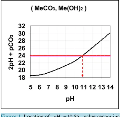
2 pH⋅ +pCO =pK_so −pK_so +2pK_W (18) The curve of y= ⋅2 pH+pCO3 vs. pH relationship is plotted in Figure 1 at CCO₃ 0.01 M

• ₌

. The numerical value of expression on the right side of Equation (18), related to defined Me+2 ion, forms a straight line parallel to pH-axis (see Figure 1). The abscissa of the point of intersection of this line with the curve y= ⋅2 pH+pCO3 vs. pH relationship indicates the pHt value, separating the pH-intervals for MeCO3 and Me(OH)2, as the

equilibrium solid phases. For example, y=23.78 calculated for the pair (ZnCO3, Zn(OH)2) corresponds to

pHt =10.85 (see Figure 1). The pHt values found this way for different Me

+2

[image:3.595.216.411.501.691.2]

ions are collected in Table 1.

Figure 1. Location of pHt=10.85 value separating

the pH-intervals for (ZnCO3, Zn(OH)2) pair (see

[image:4.595.86.542.441.665.2]

Table 1. The pH=pHt values for the systems with MeCO3

and Me(OH)2; CCO₃ 0.01 M

• ₌

; pKW =14.0.

Me2+ MeCO3 Me(OH)2

3

2pH+pCO pHt

,11

so

pK pKso,2

Cu2+ _{9.63 18.2 19.43 7.29}

Zn2+ _{10.78 15.0 23.78 10.85}

Mn2+ _{9.3 12.9 24.4 11.18}

Fe2+ 10.5 14.01 24.49 11.23

Pb2+ _{13.14 15.2 25.94 11.97}

4. Transition Points for Lead Phosphates

For Me=Pb, L=PO4

(

u=2,n=3

)

we have, among others, three solid phases: PbHPO4, Pb3(PO4)2 and

Pb(OH)2, defined by the solubility products:

(

)

2 2

4 ,11

Pb HPO pKso 11.36

+ −

= + =

4

PbHPO (19)

(

)

2 3

(

)

4 ,32

3Pb 2PO pKso 43.53

+ −

= + =

3 4 2

Pb PO (20)

(

)

2 1

(

)

,2 Pb 2OH pKso 15.2

+ −

= + =

2

Pb OH (21)

In this system, the physicochemical data related to another solid phases: Pb5(PO4)3OH and Pb4O(PO4)2 as

precipitates are also cited in literature [12] [13]; however, the solubility products for these species are formulated there in an unconventional manner. The unification of the solubility products to conventional notation will be the first, preparatory step for further considerations. The expressions for solubility products, formulated unconven-tionally, will be denoted as Kso

∗

(asterisked, with the corresponding subscripts, specifying their stoichiometric composition). We have:

(

)

1 2 3

(

)

4 2 ,531

H+ 5Pb+ 3PO− H O pK_so∗ 62.8

+ = + + =

5 4 3

Pb PO OH

(

)

1 2 3

(

)

4 2 ,422

2H 4Pb 2PO H O pKso 36.86

+ + − ∗

+ = + + =

4 4 2

Pb O PO

and then

5 3

2 3 1

4 _62.8

,531 1 1

Pb PO OH

10 H OH so K + − − ∗ − + −             = ⋅ =        

4 2 2

2 3 1

4 36.86

,422 ₁ 2 ₁ 2

Pb PO OH

10 H OH so K + − − ∗ − + −             = ⋅ =         The values:

(

)

5 3

2 3 1

,531 Pb PO4 OH ,531 ,531 76.8

so so W so

K =_ +  _{ } − _{ }  − _=K∗ ⋅K pK = (22)

(

)

4 2 2

2 3 1 2

,422 Pb PO4 OH ,422 ,422 64.86

so so W so

K =_ +  _{ } − _{ }  − _ =K∗ ⋅K pK = (23) refer to the reactions:

(

)

5Pb 2 3PO43 OH1

+ − −

= + +

5 4 3

Pb PO OH ,

(

)

2 3 1

2 4

H O 4Pb+ 2PO− 2OH−

+ = + +

4 4 2

Pb O PO (see Appendix).

At pHt, we assume (this assumption will be verified later) that the solubility products for PbHPO4 and

Pb3(PO4)2 are fulfilled simultaneously. From Equations (19), (20) and (13) we get:

H

4 ,11 ,32 1

4 4

H

PO PO ,11 ,32 1

3 pH log log 3 _{so so} 3log

y= ⋅ − C• + z = pK −pK + K (25)

where (see Equation (7))

4

12.38 pH 19.49 2pH 21.61 3pH

PO 1 10 10 10

z = + − + − + − (26)

and 2 H 3

4 4

H POi Ki H i PO

− + −

 =    

     , logK1H =12.38, H 2

logK =19.49, H 3

logK =21.61 (on the basis of [9], where pK1=2.12, pK2 =7.21, pK3=12.38). The relation (24) agrees with Equation (9), for L=PO4,

0

m= , a= = =b k 1, u= =d 2, n= =c 3. Similarly, when assuming that the solubility products for

Pb3(PO4)2 and Pb(OH)2 are fulfilled simultaneously at pH=pHt, we get:

4 ,32 ,12

3 pH⋅ +pPO =0.5pK_so −1.5pK_so +3pK_W (27) The complete set of values for y= ⋅3 pH+pPO4, related to different pairs of precipitates specified in Equa-tions (19)-(23), is presented in Table 2. Comparing the y-values in the first line of Table 2, we state that the lowest value

(

y1=27.69

)

corresponds to the pair (PbHPO4, Pb3(PO4)2); this means that Pb3(PO4)2 follows

PbHPO4 on the pH-scale. Next, considering the y-values in the second line of Table 2, we state that the

lowest y-value

(

y2=29.25

)

corresponds to the pair (Pb3(PO4)2, Pb5(PO4)3OH), i.e. Pb5(PO4)3OH is the

next precipitate on the pH-scale. Referring to the third line of Table 2, we state that the lower y-value

(

y3 =33.45

)

corresponds to the pair (Pb5(PO4)3OH, Pb4O(PO4)2), i.e. Pb4O(PO4)2 is the next precipitate on

the pH-scale. Finally, y4 =44.03 corresponds to the pair (Pb4O(PO4)2, Pb(OH)2). From the curve in Figure

1, we find the transition points pHti

(

i 1,= , 4

)

as the abscissas for y=yi

(

i 1,= , 4

)

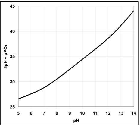
; the pHti values

separating pH intervals of the equilibrium solid phases are specified in the lower part of the Table 2. The curve of 3 pH⋅ +pPO4 vs. pH relationship is plotted in Figure 2 at CPO₄ 0.01 M

• ₌

. In particular, the curve y= ⋅3 pH+pPO4 intersects the line y= ×3 11.36−43.53 3 12.38+ × =27.69 at pHt1 =6.15, separat-ing the solid phases: PbHPO4 and Pb3(PO4)2 in pH-scale (see Table 2).

5. Crossing the pH Scale

In some cases, the precipitate of sparingly soluble salt is characterized by a relatively small solubility product value. Consequently, the pHt value, separating the pH range of the salt and the corresponding hydroxide

(

)

Me OH _u as the equilibrium solid phases, is significantly higher than the pH value, practically obtainable by addition of a strong base. In other instances, Me+u

ions form soluble hydroxo-complexes up to Me OH

(

)

+ −_pu p, characterized by the stability constant KHp value, with p=max

{ }

j >u. When pH value of the solution is

high―the hydroxide is not an equilibrium solid phase when

( )

OH 1

, Me

Me OH u p _{so u p} OH p u

p K K C

−

+ − −

 = ⋅ ⋅_ _ >

  ,

[image:5.595.90.539.528.722.2]

where CMe is the total concentration of Me in the system, Kso u, is defined by Equation (10).

Table 2. Expressions for y= ⋅3 pH+pPO4 formulated/calculated for different pairs of precipitates at the pre-assumed

pH_ti values.

Precipitate Pb3(PO4)2 Pb5(PO4)3OH Pb4O(PO4)2 Pb(OH)2

PbHPO4

,11 ,32

H 1 3

+3 log 27.69

so so pK pK K ⋅ − ⋅ = ,11 ,531 H 1

2.5 0.5 0.5

2.5 log 27.95

so W so

pK pK pK

K ⋅ − ⋅ − ⋅ + ⋅ = ,11 ,442 H 1 2 0.5

2 log 29.05

so W so

pK pK pK

K ⋅ + − ⋅ + ⋅ = ,11 H ,2 1 2 +log =36.54 so W so pK pK pK K − ⋅ −

Pb3(PO4)2

,32 ,531 5 3 3 29.25 so so W pK pK pK ⋅ − ⋅ + ⋅ = ,32 ,442 2 3 1.5 31.77 so W so pK pK pK ⋅ + ⋅ − ⋅ = ,32 ,2 0.5 3 1.5 40.965 so W so pK pK pK ⋅ + ⋅ − ⋅ =

Pb5(PO4)3OH

,531 ,442 0.5 3 2.5 33.45 so W so pK pK pK ⋅ + ⋅ − ⋅ = ,531 ,2

1 3 3

3 4 42.27

so W so pK pK pK ⋅ + ⋅ − ⋅ =

Pb4O(PO4)2

,422 ,2 0.5 3 2 44.03 so W so pK pK pK ⋅ + ⋅ − ⋅ =

PbHPO4 Pb3(PO4)2 Pb5(PO4)3OH Pb4O(PO4)2 Pb(OH)2

1

As an example, let us take the precipitates: ZnS

(

pKso1=24.7

)

and Zn(OH)2

(

pKso2=15.0

)

. Applying

2

S S S 0.01

C•=_ − _⋅f = , fS 1019.97 2pH 1012.92 pH 1

− −

= + + ( pK1=7.05 and pK2 =12.92 for dissociation con-stants K1 and K2 of H S2 ), we get y=2pH+pS= pKso1−pKso2+2pKW =24.37 15.0− + ×2 14=37.37.

The pH=pHt as abscissa related to this y-value is much higher than 14 (see Figure 3); what is more, it is

much higher than pH values of a saturated strong base. Moreover, at high pH values, Zn(OH)2 is

trans-formed into soluble complexes, mainly Zn OH

( )

₄−2

(

p= >4 2

)

.

Another example is the system with precipitates: CaC2O4

(

pKso11=8.64

)

and Ca(OH)2

(

pKso2 =5.26

)

.

Applying CC O_{2 4} C O2 42 fC O_{2 4} 0.01 • _= − _{⋅ =}

  , fC O_{2 4} 105.52 2pH 104.27 pH 1

− −

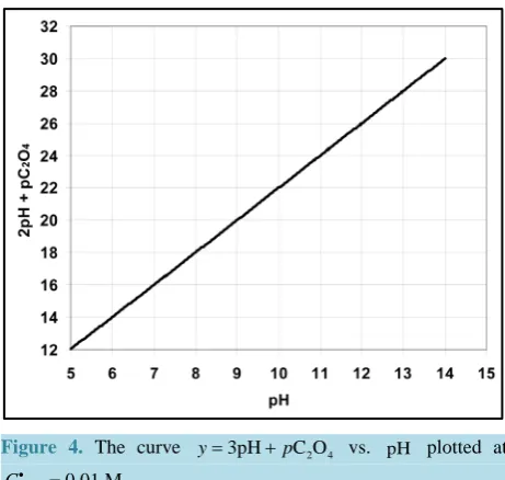
= + + (pK1=1.25, pK2 =4.27 for dis-sociation constants K1 and K2 of H2C2O4), we get y=2pH+pC O2 4 = 2pKso11−pKso2+ pKW =31.38 (see

Figure 4); this value corresponds to pHt =14.69, related to calculated pH value of 4.9 mol/L NaOH. The

Ca(OH)2 does not dissolve in an excess of strong base; Ca+2 forms only one hydroxo-complex, CaOH+1

(

p= <1 2

)

, and then Ca(OH)2 is not dissolved in an excess of OH−1 ions.

Figure 2. The curve y= ⋅3 pH+pPO₄ vs. pH, plotted at

4

PO 0.01 M

C• = .

Figure 3. The curve y=3pH+pS vs. pH plotted at

S 0.01 M

C•= .

20 22 24 26 28 30 32

5 6 7 8 9 10 11 12 13 14 15

pH

2

p

H

+

[image:6.595.197.430.238.447.2] [image:6.595.196.431.287.704.2]

Figure 4. The curve y=3pH+pC O_{2 4} vs. pH plotted at

24

C O 0.01 M

C• = .

6. Final Comments

A simple, uniform method for determining the pH ranges of different precipitates as the equilibrium solid phases in aqueous systems with Me- and L-species is presented. The systems with two or more precipitates thus formed are discussed, together with the problem of ordering of appropriate precipitates along the pH scale. The above issues are applicable to the systems where soluble complexes of the Mea

(

H Lk

)

bau b n k( )

+ − −

and/or

( )

Me OH Lcu m dn

c m d

+ − −

type are not formed or are relatively weak ones.

Solubility products can be defined in different ways. The lack of awareness of this fact can be a source of confusion, as results from examples taken from the literature. In particular, for the solubility product Kso11 of

PbHPO4 we find the following pKso11 values: 11.36 [14], and ···23.80 [15]―both are referred allegedly to the

dissociation reaction 2 2

4

Pb+ HPO−

= +

4

PbHPO . The third value, which we denote as pKso

∗

, is significantly different from the previous ones; we can therefore assume that, in fact, it relates to dissociation reaction

2 1 3

4

Pb +H+ + PO−

= +

4

PbHPO . Indeed, after introducing the dissociation constant K3 concerning the reaction

2 1 3

4 4

HPO− =H+ +PO−

(

pK₃=12.38

)

, we get pKso11 pKso11 pK3 23.80 12.38 11.42

∗

= − = − = , i.e., the value

close to 11.36. The solubility product for Pb5(PO4)3OH is also formulated improperly in [15].

References

[1] Michałowski, T. and Pietrzyk, A. (2006) A Thermodynamic Study of Struvite + Water system. Talanta, 68, 594-601.

http://dx.doi.org/10.1016/j.talanta.2005.04.052

[2] Michałowski, T. and Asuero, A.G. (2012) Thermodynamic Modeling of Dolomite Behavior in Aqueous Media.

Jour-nal of Thermodynamics, 2012, Article ID 723052.

http://www.hindawi.com/journals/jtd/2012/723052/cta/

[3] Michałowski, T. (2011) Application of GATES and MATLAB for Resolution of Equilibrium, Metastable and Non-

Equilibrium Electrolytic Systems. In: Michałowski, T., Ed., Applications of MATLAB in Science and Engineering,

Chapter 1, InTech, Rijeka, 1-34.

http://www.intechopen.com/books/show/title/applications-of-matlab-in-science-and-engineering

[4] Michałowski, T. and Lesiak, A. (1994) Formulation of Generalized Equations for Redox Titration Curves. Chemia

Anali-Tyczna (Warsaw), 39, 623-637.

[5] Michałowski, T., Ponikvar-Svet, M., Asuero, A.G. and Kupiec, K. (2012) Thermodynamic and Kinetic Effects

In-volved with pH Titration of As(III) with Iodine in a Buffered Malonate System. Journal of Solution Chemistry, 41,

436-446. http://dx.doi.org/10.1007/s10953-012-9815-6

[6] Michałowski, T., Asuero, A.G., Ponikvar-Svet, M., Toporek, M., Pietrzyk, A. and Rymanowski, M. (2012) Principles

of Computer Programming Applied to Simulated pH-Static Titration of Cyanide According to a Modified Liebig-De-

[image:7.595.197.428.82.301.2]

[7] Michałowski, T., Toporek, M., Michałowska-Kaczmarczyk, A.M. and Asuero, A.G. (2013) New Trends in Studies on

Electrolytic Redox Systems. Electrochimica Acta, 109, 519-531. http://dx.doi.org/10.1016/j.electacta.2013.07.125

[8] Michałowski, T., Michałowska-Kaczmarczyk, A.M. and Toporek, M. (2013) Formulation of General Criterion

Distin-guishing between Non-Redox and Redox Systems. Electrochimica Acta, 112, 199-211.

http://dx.doi.org/10.1016/j.electacta.2013.08.153

[9] Michałowski, T. (1982) Solubility Diagrams and Their Use in Gravimetric Analysis. Chemia Analityczna, 27, 39.

[10] Dirkse, T.P., Michałowski, T., Akaiwa, H. and Izumi, F. (1986) Copper, Silver, Gold and Zinc, Cadmium, Mercury

Oxides and Hydroxides. Pergamon Press, Oxford.

http://search.library.wisc.edu/catalog/ocm12945958

[11] Michałowski, T., Janecki, D., Lechowicz, W. and Meus, M. (1996) pH Intervals for Precipitates in Two-Phase Systems.

Chemia Analityczna (Warsaw), 41, 687-695.

[12] Crannell, B.S., Eighmy, T.T., Krzanowski, J.E., Eusden Jr., J.D. Shaw, E.L. and Francis, C.A. (2000) Heavy Metal

Stabilization in Municipal Solid Waste Combustion Bottom Ash Using Soluble Phosphate. Waste Management, 20,

135-148. http://dx.doi.org/10.1016/S0956-053X(99)00312-8

[13] Viellard, P. and Tardy, Y. (1984) Thermochemical Properties of Phosphates. In: Nriagu, J.O. and Moore P.B., Eds.,

Phosphate Minerals, Springer-Verlag, Berlin, 171-198. http://dx.doi.org/10.1007/978-3-642-61736-2_4

[14] Inczédy, J. (1976) Analytical Applications of Complex Equilibia. Horwood, Chichester.

[15] Saisa-ard, O. and Haller, K.J. (2012) Crystallization of Lead Phosphate in Gel Systems. Engineering Journal, 16, 161-

168. http://dx.doi.org/10.4186/ej.2012.16.3.161

Appendix

As an example, let us consider the pair of precipitates defined by Equations (22) and (23). We have, by turns,

(

)

5 3 20 12 4 4

2 3 1 2 3 1

4 531 4 531

Pb PO OH Kso Pb PO OH Kso

+ − − + − −

     = →      =

           

(

)

4 2 2 20 10 10 5

2 3 1 2 3 1

4 ,422 4 ,422

Pb+ PO− OH− K_so Pb+ PO− OH− K_so

      = →      =

           

(

)

(

)

20 12 4 4

2 3 1

4 ,531

20 10 10 5

2 3 1

,422 4

Pb PO OH

Pb PO OH

so

so K K

+ − −

+ − −

           _{ =}            

(

)

(

)

(

(

)

)

2 4 2

3 3

4 ,531 4 ,531

6 5 3 2.5

1 1

,422 ,422

PO PO

OH OH

so so

so so

K K

K K

− −

− −

   

  _{= →}   ₌

   

   

(

)

(

)

(

)

( )

(

)

3 2 2 3

3 1

3

4 ,531 1 3 ,531

4

3 3 2.5 2.5

1 1

,422 ,422

PO H

H PO

OH H

so so W

so so

K K K

K K

− +

+ −

− +

    ⋅

  _⋅  _{= →   =}        

   

4 ,531 ,422