Satellite Image Compression using Fractional Fourier Transform

Satellite Image Compression using Fractional Fourier

Transform

Rajinder Kumar

Research Scholar, Dept. of ECE Thapar University, Patiala

Kulbir Singh

Associate Professor, Dept. of ECE Thapar University, Patiala

Rajesh Khanna

Professor & Head Dept. of ECE Thapar University, Patiala

ABSTRACT

The Fourier transform can be successfully used in the field of signal processing, image processing, communications and data compression applications. The discrete fractional Fourier transform, generalization of the discrete Fourier transform, is used for compression of high resolution satellite images. With the extra degree of freedom provided by the DFrFT, its fractional order „a‟, high visual quality decompressed image can be achieved. Different satellite images of size 512×512 and 256×256 are studied and performance parameters such as peak signal-to-noise ratio (PSNR), mean square error (MSE) and compression ratio (CR) are determined.After subdivide the images, DFrFt is applied to obtain the transformed coefficients for calculating PSNR and IDFrFt is applied for reconstruction of satellite images. It is analyzed that by changing the value of fractional order „a‟ to different value, the DFrFT can achieved minimum MSE and corresponding maximum PSNR between 0.8 to 1 fractional order for same amount of CR. It is observed that discrete fractional Fourier transform is very efficient for obtaining better PSNR around 41 dB at 50% CR while maintaining the higher visual quality of decompressed satellite images. The significant improvement is observed using DFrFT as compare to existing classical lifting scheme for satellite image compression based on discrete wavelet transform (DWT).

General Terms

Satellite Image Compression, Fractional Transform

Keywords

Satellite Image Compression, DFrFT, PSNR, MSE

.

1.

INTRODUCTION

The images captured by the new generation satellites are remotely sensed image used in weather reporting, regional planning, global positioning system, etc., also including fields of education welfare and intelligence as well [1]. These remotely sensed image data is to be communicated from remote area to receiver station, are facing with problem of storage and transmission of imagery data because of limited bandwidth, time of data transmission and increase in spatial resolution. Today most of the satellites are operates on store-and-forward criterion; i.e. imagery is captured, stored on satellite, transmitted to ground station .This had increase the hunger demand on storage because of lager volume of data is collected by high resolution satellite imagery system and requires more downlink time to transmit them to earth station. Due to stringent requirement on bandwidth and storage capacity, the satellite image data need to be compressed before it send to earth station while preserving the high visual quality of the decompressed image. It has been noticed that FrFT is popularly used in the field of image processing. The fractional Fourier transform (FrFT), which is a generalization

of the ordinary Fourier transform (FT), introduced to quantum mechanics by Namias in 1980 [2], then rediscovered in optics [4]-[6] and introduced to the signal processing community by Almeida in 1994 [3]. The continuous fractional Fourier transform (FrFT) represents a rotation of signal in time-frequency plane as discuss by various authors [3]-[6]. Santhanam and McClellan [7] first reported the work on discrete version of fractional Fourier transform in 1995. The DFrFT based on eigen-decomposition of DFT kernel matrix [9] introduced by S.C. Pei in 1996 [8]. After that the DFrFT redefined by C. Candanet al. in 2000 [11]. The significant feature of fraction Fourier domain image compression benefits from its extra degree of freedom that is provided by its fractional orders. The FrFT share many useful properties of the regular Fourier transform and has a free parameter „a‟, its fraction. When the fraction is zero, we get the Fourier modulated version of the input signal. When it is unity, we get the conventional Fourier transform. As the fraction changes from 0 to 1 we get different forms of the signal, which interpolate between the Fourier modulated form of the signal and its FT representation. In this paper, the satellite images are compressed by discrete fractional Fourier transform. The paper is organized as follows: The definition of discrete fractional Fourier transform (DFrFT) and some properties of DFrFT are presented in sections 2. In section 3, presents the satellite image compression using DFrFT. In section 4, presents the results and conclusion is discuss in section 5.

2.DISCRETE FRACTIONAL FOURIER

TRANSFORM

The FrFT belongs to the class of time–frequency representations that have been extensively used by the signal processing community. In all the time–frequency representations, one normally uses a plane with two orthogonal axes corresponding to time and frequency.The computation of DFrFT is based upon the eigen-decomposition of the DFT kernel matrix [8]. The kernel matrix of DFT has only four distinct eigenvalues [l, - j, -1, j] shown in [9]. The eigenvectors construct a vector space same eigenvalue because these eigenvectors of DFT kernel are not uniquely determined. A matrix S to evaluate the eigenvectors of F with real values [13]. The matrix S is defined as follows:

𝐒 =

𝟐 𝟏 𝟎

𝟏 𝟐𝒄𝒐𝒔𝝎 𝟏 𝟎 𝟏 𝟐𝒄𝒐𝒔𝟐𝝎

𝟎 … 𝟏 𝟎 … 𝟎 𝟏 … 𝟎 ⋮ ⋮ ⋮

𝟏 𝟎 𝟎 ⋱

𝟎 … 𝟐𝐜𝐨𝐬⁡(𝑵 − 𝟏)𝝎

whereω= 2𝜋_𝑁. It satisfies the following commutative property.

The eigenvectors of S matrix are same as that of the eigenvectors of F having different corresponding eigenvalues. Due to symmetric property of S matrix, all eigenvalues of S matrix are real and the eigenvectors are orthonormal each other. The eigen-decomposition of matrix S is written as: 𝐒 = 𝑁−1𝑘=0𝛾𝑘𝒗𝒌 (2) where𝒗𝒌 is the eigenvector of the matrix S corresponding to the eigenvalue 𝛾𝑘. The eigen-decomposition of DFT kernel matrix F is written as:

𝐅 = 𝒗𝒌𝒗𝒌∗ + (−𝑗)𝒗𝒌𝒗𝒌∗ 𝑘∈𝐸2

𝑘∈𝐸1

+ (−1)𝒗𝒌𝒗𝒌∗ 𝑘∈𝐸3

+ (𝑗)𝒗𝒌𝒗𝒌 ∗ 𝑘∈𝐸4

(3)

whereE1,E2,E3 and E4 is the set of indices for eigenvectors belongs to eigenvalues [l, - j, -1, j ] respectively. From equation 3 the eigenvalues of DFT kernel is determined. By taking fractional powers of these eigenvalues, the transform kernel of DFrFT can be easily defined as

𝑹𝜶 _{= 𝑭}𝟐𝜶_𝝅

𝒆−𝒋𝑵𝜶_𝒗 𝒌𝒗𝒌∗ 𝑵−𝟏

𝒌=𝟎

𝐍𝐢𝐬𝐨𝐝𝐝

𝒆−𝒋𝑵𝜶_𝒗

𝒌𝒗𝒌∗+ 𝒆−𝒋𝑵𝜶𝒗𝑵−𝟏𝒗𝑵−𝟏∗ 𝐍𝐢𝐬𝐞𝐯𝐞𝐧 𝑵−𝟐

𝒌=𝟎

where𝒗𝒌is the eigenvector obtained from matrix S. The DFrFT of signal x(n)can be computed through equation

𝑋𝛼 𝑛 = 𝑹𝜶𝑥 𝑛 = 𝑭 𝟐𝜶

𝝅𝑥 𝑛 = 𝑽𝑫 𝟐𝜶

𝝅𝑽∗𝑥(𝑛)(4) The signal x(n) can also be recovered from its DFrFT through anoperation with parameter (-α) as

𝒙 𝒏 = 𝑹−𝜶𝑿𝜶 𝒏 = 𝑽𝑫 −𝟐𝜶

𝝅 𝑽∗𝑿_𝜶(𝒏)₍₅₎ Some properties of DFrFT are discuss in Table 1

Table 1.Properties of DFrFT

1. Unitary 𝑹𝜶∗ = 𝑹𝜶−𝟏= 𝑹−𝜶 2. Angle Additivity 𝑹𝜶𝑹𝜷= 𝑹𝜶+𝜷 3. Time inversion 𝑹𝜶𝒙 −𝒏 = 𝑿𝜶 −𝒏

4. Periodicity 𝑹𝜶+𝟐𝝅= 𝑹𝜶

5. Symmetric 𝑹𝜶 𝒂, 𝒃 = 𝑹𝜷 𝒃, 𝒂 The above definition of DFrFT is applicable for one dimensional signals such as speech waveform. For analysis of two-dimensional (2D) signals such as images, we need a 2D version of the DFrFT. For an MN matrix, the 2D DFrFT is computed in a simple way: The 1D DFrFT is applied to each row of matrix and then to each column of the resultant matrix. The 2D transformation kernel is defined with separable form as [10]:

𝑹(𝜶,𝜷)= 𝑹𝜶⊗ 𝑹𝜷

The 2D forward and inverse DFrFT are computed from above 2D transformation kernel as:

𝑋 𝛼,𝛽 𝑚, 𝑛 = 𝑥 𝑝, 𝑞 𝑵−𝟏

𝒒=𝟎 𝑴−𝟏

𝒑=𝟎

𝑹 𝜶,𝜷 𝒑, 𝒒, 𝒎, 𝒏

𝑥 𝑝, 𝑞 = 𝑋 𝛼,𝛽 𝑚, 𝑛 𝒏=𝟎

𝒎=𝟎

𝑹 −𝜶,−𝜷 (𝒑, 𝒒, 𝒎, 𝒏)

In two-dimensional DFrFT we have to consider two angles of rotation =a/2 and =b/2 and If one of these angles is zero, the 2D transformation kernel reduces to the 1D transformation kernel.

3. SATELLITE IMAGE COMPRESSION

USING DFRFT

In satellite image processing, an important part is the compression. This means the reducing the dimensions of the images, to a level that can be easily used or processed. Image compression using transform coding yields extremely good compression, with controllable degradation of image quality [12]. By adjusting the cutoff of the transform coefficients, a compromise can be made between image quality and compression factor. To exploit this method, an image is first partitioned into non-overlapped nn(generally taken as 8x8 or 1616) sub images as shown in figure 1. A 2D-DFrFT is applied to each block to convert the gray levels of pixels in the spatial domain into coefficients in the frequency domain. The coefficients are normalized by different scales according to the cutoff selected. At decoder simply inverse process of encoding by using inverse 2D-DFrFT is performed. The Peak Signal-to-Noise Ratio (PSNR) value used to measure the difference between a decoded imageg(i, j) and its original imagef(i,j) is defined as follows. In general, the larger PSNR value, the better will be decoded image quality.

   





1 0 1 0 , , 1



MSE (6)

dB MSE

PSNR10log_10255255_ (7)

where MN is the size of the images, g(i, j)andf (i, j) are the matrix elements of the decompressed and original images at (i,j)pixel. Another parameter known as compression ratio used in this compression technique and it is defined as the ratio of size compressed image to the size of original image and is given below:

CR % =Size of Compressed Image Size of Original Image × 100

4. RESULTS

Input image

N×N Compressed image

(a)

Compressed images Decompressed Images

(b)

Figure1: Satellite image compression model (a) Encoder; (b) Decoder

(a) (b)

(c) (d)

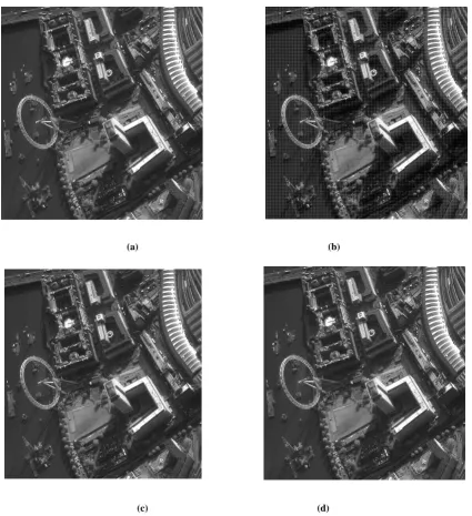
Figure 2: Satellite image 1 of 512x512 at 50% CR (a) Original image, (b) Decompressed image at fractional order 0.5, (c) Decompressed image at optimum fractional order 0.86, (d) Decompressed image at fractional order 1

Merge n × n sub-images IDFrFT

Construct n ×n

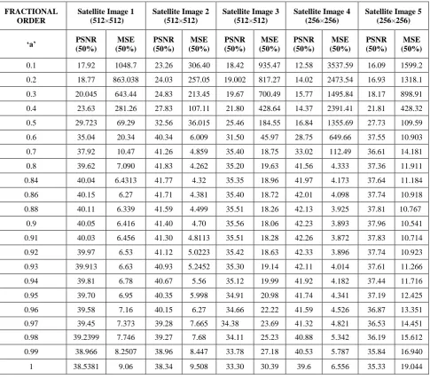
Table 2. Results of five different satellite images of size 256×256 and 512×512 at 50% CR

(a) (b)

FRACTIONAL ORDER

Satellite Image 1 (512×512)

Satellite Image 2 (512×512)

Satellite Image 3 (512×512)

Satellite Image 4 (256×256)

Satellite Image 5 (256×256) ‘a’ PSNR

(50%)

MSE (50%)

PSNR (50%)

MSE (50%)

PSNR (50%)

MSE (50%)

PSNR (50%)

MSE (50%)

PSNR (50%)

MSE (50%)

0.1 17.92 1048.7 23.26 306.40 18.42 935.47 12.58 3537.59 16.09 1599.2 0.2 18.77 863.038 24.03 257.05 19.002 817.27 14.02 2473.54 16.93 1318.1 0.3 20.045 643.44 24.83 213.45 19.67 700.49 15.77 1495.84 18.17 898.91 0.4 23.63 281.26 27.83 107.11 21.80 428.64 14.37 2391.41 21.81 428.32 0.5 29.723 69.29 32.56 36.015 25.46 184.55 16.84 1355.69 27.73 109.59

0.6 35.04 20.34 40.34 6.009 31.50 45.97 28.75 649.66 37.55 10.903

0.7 37.92 10.47 41.26 4.859 35.40 18.75 33.02 112.49 36.61 14.181

0.8 39.62 7.090 41.83 4.262 35.20 19.63 41.56 4.333 37.36 11.911

0.84 40.04 6.4313 41.77 4.32 35.35 18.96 41.97 4.173 37.64 11.184

0.86 40.15 6.27 41.71 4.381 35.40 18.72 42.01 4.098 37.74 10.918

0.88 40.11 6.339 41.59 4.499 35.51 18.26 42.13 3.925 37.81 10.767

0.9 40.05 6.416 41.40 4.70 35.56 18.06 42.23 3.893 37.96 10.541

0.91 40.03 6.456 41.30 4.8113 35.51 18.28 42.26 3.872 37.83 10.714

0.92 39.97 6.53 41.12 5.0223 35.42 18.63 42.33 3.896 37.74 10.923

0.93 39.913 6.63 40.93 5.2452 35.30 19.14 42.11 4.014 37.61 11.266

0.94 39.81 6.78 40.67 5.56 35.12 19.99 41.92 4.182 37.44 11.716

0.95 39.70 6.95 40.35 5.998 34.91 20.98 41.74 4.341 37.19 12.425

0.96 39.58 7.16 40.15 6.27 34.66 22.22 41.59 4.526 36.87 13.351

0.97 39.45 7.373 39.28 7.665 34.38 23.69 41.32 4.821 36.53 14.451

0.98 39.2399 7.746 39.27 7.68 34.11 25.23 40.88 5.342 36.19 15.612

0.99 38.966 8.2507 38.96 8.447 33.78 27.18 40.53 5.787 35.84 16.940

(c) (d)

Figure 3: Decompressed satellite image 1 of 512x512 at optimum fractional order ‘a’ (a)Image Quality at 10% CR with ‘a’=0.84, (b) Image Quality at 30% CR with ‘a’=0.88, (c) Image Quality at 50% CR with ‘a’=0.86, (d) Image Quality at 70%

CRwith ‘a’=0.94

givesgood visual quality of satellite image.

Decompressed Image quality at different compression ratio with optimum fractional order „a‟ in which the best quality of images are obtained shown in figure 3. The plots of MSE and PSNR versus changing fractional order ofDFrFT at different compression ratio for satellite image 1 has been calculated and depicted in figure 4 and 5.Table 2 shows the results in terms of PSNR and MSE of five different satellite images at 50% CR.

Figure 4: Peak Signal-to-Noise Ratio(dB) versus fractional order

It is clear from table 2 that at „a‟=0.5, MSE is 69.29 but as „a‟ increase to 0.86, MSE decrease upto 6.27, PSNR increase to 40.15 dB. After that again MSE increases with increase in „a‟. When „a‟=1 FrFT become conventional FT, corresponding MSE=9.06 and PSNR=38.53 dB.Figure 6 show closed view

of the variation of MSE with fractional order „a‟. Generally,

Figure 5: Mean Square Error versus fractional order

Figure 6: Mean Square Error versus fractional order

0.1 0.2 0.3 0.4 0.5 0.6 0.7 0.8 0.9 1

15 20 25 30 35 40 45 50 55 60 65

Frational Order of DFRFT

P

S

N

R

(

d

B

)

Peak Signal-to-Noise Ratio at different Compression Ratio 10% CR

20% CR 30% CR 40% CR 50% CR 70% CR

0.1 0.2 0.3 0.4 0.5 0.6 0.7 0.8 0.9 1 0

500 1000 1500 2000 2500

Frational Order of DFRFT

M

S

E

MeanSquare Error at different Compression Ratio 10% CR 20% CR 30% CR 40% CR 50% CR 70% CR

0.8 0.82 0.84 0.86 0.88 0.9 0.92 0.94 0.96 0.98 1 0

5 10 15 20 25 30 35

Frational Order of DFRFT

M

S

E

MeanSquare Error at different Compression Ratio

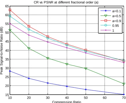
Figure 7: PSNR (dB) versus Compression Ratio(CR)

there is tradeoff between image quality and CR. As CR increases, PSNR decreases and image quality degrades for constant fractional order „a‟ shown in figure 7.

5. COMPARISON WITH CLASSICAL

LIFTING SCHEME

The classical lifting scheme is discrete wavelet transform based image compression techniques for high resolution satellite images [16]. By using this techniques,the maximum PSNR around 29 dB is obtained and compression ratio 8. By using purposed scheme, the maximum PSNR around 41 dB at 50% CR is achieved.

6. CONCLUSION

It is conclude that, a technique for Satellite image compression using DFrFT makes the full use of the additional degrees offreedom provided by the fractional orders to achieve an optimum domain for which CR is more, MSE is less and better PSNR, also good image quality is retained. It is clear that significant improvement in PSNR and CR using DFrFT over the classical lifting scheme for satellite image compression. It also observed that with increases in CR the quality of image is decreases.

7. REFERENCES

[1] Nair,G.M. 2008. “Role of communications satellites in national development”, IETE Technical Review, vol. 25, 3-8.

[2] Namias, V. 1980. "The fractional order Fourier transform and its application to quantum mechanics", Journal of Institute of Mathematics and its Applications,no. 25, 241-265.

[3] Almeida,L. B. 1994."The fractional Fourier transform and time-frequency representations", IEEE Transactions on Signal Processing, vol. 42, no.11, 3084-3091, (Nov1994).

[4] Mendlovic,D. and. OzaktasH. M. 1993."Fractional Fourier transforms and their optical implementation: I", Journal of the Optical Society of America A, vol. 10, no. 9, 1875-1881, (Sept. 1993).

[5] Ozaktas,H. M. andMendlovic, D. 1993. "Fractional Fourier transforms and their optical implementation: II", Journal of the Optical Society of America A, vol. 10, no. 12, 2522-2531, (Dec. 1993).

[6] Alieva,T., Lopez,V.,Agullo-Lopez,F. and Almeida, L. B. 1994. "The fractional Fourier transform in optical propagation problems", Journal of Modern Optics, vol. 41, no. 5, 1037-1044, (May 1994).

[7] Santhanam, B. and McClellan,J. H. 1995."The DFrFT-A Rotation in Time Frequency Space", IEEE Trans. on Signal Processing, vol. 5, 921–923.

[8] Pei, S.C. andYeh, M. H. 1996. "Discrete fractional Fourier transform" IEEE International Symposium onCircuits and Systems,vol. 2, 536 – 539.

[9] McClellan, J. H. and Parks,T. W. 1972. "Eigenvalue and eigenvector decomposition of the discrete Fourier transform", IEEE Transaction on Audio and Electroacoustics, AU-20, 66-74, (Mar. 1972).

[10]Pei, S.C.andYeh, M. H. 1998."Two dimensional discrete fractional Fourier transform", Signal Processing, vol. 67, 99-108.

[11]Candan,C., Kutay, M. A.and Ozaktas,H. M. 2000. "Discrete fractional Fourier Transform", IEEE Transactions on Signal Processing, vol. 48, no. 5, (May 2000).

[12]Yetik, I. S., Kutay, M.A. and Ozaktas,H.M. 2001."Image representation and compression using fractional Fourier transform", Optical Communication., vol. 197, 275-278. [13]Dickinson,B. W. and Steiglitz,K. 1982."Eigenvectors and

functions of the discrete Fourier transform", IEEE Transaction Acoustic., Speech, and Signal Processing., vol. ASSP-30, 25-31, (Feb. 1982).

[14]Said and Pearlman, A. 1996."An Image Multiresolution Representation for Losssless and Lossy Compression", IEEE Transaction on Image Processing, vol. 5, no. 9, 243-250, (Sep. 1996).

[15] Shapiro,J.M. 1993. "Embedded Image Coding Using Zerotrees of Wavelet Coefficients", IEEE Transaction on Signal Processing, vol. 41, 3445-3462.

[16] Nagmani,K. and Anant, A.G. 2011. "Image Compression Techniques for High ResolutionSatellite Imageries using Classical Lifting Scheme", International Journal of Computer Applications, vol. 15, no. 3, 25-28, (Feb. 2011).

[17]Usevitch, B. 2001."A Tutorial on Modern Lossy Wavelet Image Compression: Foundations of JPEG 2000", IEEE Signal Processing Magazine.

10 20 30 40 50 60 70 15

20 25 30 35 40 45 50 55 60 65

Compression Ratio

P

e

a

k

S

ig

n

a

l-to

-N

o

is

e

R

a

ti

o

(

d

B

)

CR vs PSNR at different fractional order (a)