Identification of MIMO Hammerstein models using
Singular Value Decomposition approach
Badreddine Louhichi
Laboratory of Sciences and Techniques of Automatic control & computer engineering. National School of Engineering of Sfax,
University of Sfax
Ahmed Toumi
Laboratory of Sciences and Techniques of Automatic control & computer engineering. National School of Engineering of Sfax,
University of Sfax
ABSTRACT
In this paper, we present a new approach to identify multivariable Hammerstein systems based on the Singular Value Decomposition (SVD) method. The technique allows for the determination of the memoryless static nonlinearity as well as the estimation of the model parameters of the dynamic Auto-Regressive model with eXogenous input (ARX) part. First of all, an iteration procedure is proposed to identify the parameters of Multi-Input Multi-Output (MIMO) Hammerstein models by using the Recursive Least Squares (RLS) algorithm. Secondly, the obtained parameter estimates of the identification model include the product terms of the parameters of the original systems. So, to separate these parameters of the original parameters from the product terms, the singular value decomposition method is discussed. Finally, a simulation study is performed to demonstrate the effectiveness of the proposed method compared with the existing approaches.
General Terms
Hammerstein systems, System identification.
Keywords
MIMO Hammerstein systems, Parameter estimation, Singular value decomposition method, Recursive least squares algorithm, Non linear systems.
1.
INTRODUCTION
Transfer function models are used for design of control systems for mildly nonlinear systems. However, for highly nonlinear systems, the controller design based on the linear model may not be adequate. For such cases, the linear model based on a fixed controller will not give a satisfactory response. Indeed, a suitable nonlinear model representation will be desirable [16]. Two of the most frequently studied nonlinear systems are the Hammerstein and Wiener models where the nonlinear block is static and follows or followed by a linear system. A Hammerstein model consists of static nonlinear block followed by a linear dynamic block, and a Wiener model consists of linear dynamic block followed by a static nonlinear function.
To identify the Hammerstein model, a various system identification methods have been proposed in the literature. However, most of the methods focus on Input Single-Output (SISO) processes [4 – 10, 32]. The first work which developed an iterative identification procedure for Hammerstein model is presented by Narendra et al. [26].
Recently, to guarantee the global convergence of the model parameters in an iterative manner [14] developed an updating algorithm based on the Lyapunov approach. In addition, several approaches have been proposed to identify Hammerstein models in a non-iterative fashion. For examples Pottmann et al. in [27] proposed a two-stage identification algorithm to extract the model parameters. To separate the identification of the linear dynamic part from that of the static nonlinear part, Sung in [29] used a special test signal. Laksminarayanan et al. in [19] proposed multivariate statistical tools to identify the Hammerstein models. Al-Duwaish et al. in [2] used an hybrid model consisting of a neural network to identify the static nonlinear part in series with Auto-Regressive Moving Average (ARMA) model for identification of SISO and Multi-Input Multi-Output (MIMO) Hammerstein models. Several other identification and controller design methods for Hammerstein models were developed by [1, 20, 30].
For Hammerstein systems, the parameters from the identification model include the products of the original system parameters [3, 25], so separating the original parameters from the obtained parameter estimates of the product terms is required. The authors in [6 – 9] proposed a simple average method of separating parameters for Hammerstein models. Another separating parameter method is the singular value decomposition done by Bai in [3]. This paper presents an algorithm for identification of MIMO Hammerstein nonlinear systems by using the Recursive Least Squares (RLS) with an exponential forgetting factor and uses the singular value decomposition method to separate the system estimated parameters.
The paper is organized as follows. Section 2 describes the system formulation related to the MIMO Hammerstein models. Section 3 presents an identification algorithm to estimate the parameters of the system. Section 4 introduces a separating parameter method. The main results are given in section 5. Section 6 gives some conclusions.
2.
PROBLEM FORMULATION
Two possible structures as depicted in figures 1 and 2 can be used to describe a MIMO Hammerstein model depending on whether the nonlinearities are separate or combined [2, 19]. The combined nonlinearity case is more general, but it can cause a very challenging parameter estimation problem because of the large number of parameters to be estimated [11]. Therefore, the MIMO Hammerstein model with separate nonlinearities will be considered in this paper (figure 2). As mentioned previously, the system consists of a static part which contains all the nonlinearity followed by a Linear Time Invariant (LTI) model
H q
(
1)
which contains all the dynamics of the process.where
1
u
,
1
y
T T
n n
U k u k u k Y k y k y k
and
1
y
T n
E k e k e k are the system input, output and white noise with zero mean at time k respectively
.
fi(.) are polynomials of a known order in the input as follows :
1
2 2
mi mi
i i i i i i i
f k u k u k u k (1)
where 1 2
, , , mi
i i i
present the nonlinear system parameters.
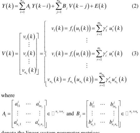
Assume that the LTI system has the Auto-Regressive with eXogenous input (ARX) structure (but other structure like Auto-Regressive Moving Average with eXogenous input (ARMAX), Auto-Regressive Integrated Moving Average with eXogenous input (ARIMAX) etc. are also possible). The input– output relationship is then given by :
1 1
A B
n n
i j
i j
Y k A Y k i B V k j E k
(2)
1
1 1 1 1 1
1 1
1
1
i
u nu
u u u u u
m r r r m
r r i i i i i i
r
n m
r r n n n n n
r
v k f u k u k
v k
v k v k f u k u k
V k
v k
v k f u k u k
(3)
where
11 1 11 1
x x
1 1
and
y u
y y y u
y y y y y u
i i j j
n n
n n n n
i j
i i j j
n n n n n n
a a b b
A B
a a b b
denote the linear system parameter matrices.
Assume that for k ≤ 0, uj(k) = 0, yj(k) = 0 and ej(k) = 0 for
j {1, …, ny} and nA, nB, mj for j {1, …, nu}, ny and nu
represent the order of the output, the order of the input, the order of the nonlinearity, the number of outputs and the number of inputs respectively.
This paper presents an identification algorithm to estimate the parameters i
k j
a , i k j
b and r i
of the system in (2) from given input – output data {ui(k), yi(k)} and to evaluate the
[image:2.595.314.538.251.464.2]accuracy of the estimated parameters by simulation on computers.
Fig 1 : MIMO Hammerstein model with combined
nonlinearities.
1H q f(.)
v1(k)
v2(k)
un
v k
y1(k)
y2(k)
yn
y k
u1(k)
u2(k)
un
[image:2.595.74.270.441.546.2]u k
Fig 2 : MIMO Hammerstein model with separate
nonlinearities. H q
1 v1(k)v2(k)
un
v k
y1(k)
y2(k)
yn
y k
u1(k)
u2(k)
un
u k
f1(.)
f2(.)
The ith output equation from system (2) can be written as follows :
1 2 1 2 1 1 2 21 1 1
1 1 1
1 1 1 1
1 1 1 2 2 2 2 2 2
1 1 1
2 1 2 2 1
1 1 1 1 1 1 2 2 2
2 2
2 2 2
1 1
1 1 1
+ 1 1
2 2 2
2 +
A
nu nu
u u u u u u
u
n
i i i A i
m m
m m
i i i
m m
i n n n i n n n m m
i i i
m m
i i n n
y k A Y k A Y k n b u k
b u k b u k b u k
b u k b u k
b u k b u k b u k
b u k b
1 1 2 2 1 2 11 1 1 1
1 1 1 2 2 2
1 2 2 2
2 2 + u u nu nu B
u u u
B B
B B
u u u
nu nu
B
u u u
n m
m n
i n n n i B m
n m n
i B i B
m
n m n
i B i n n n B m
m n
i n n n B
u k
b u k b u k n
b u k n b u k n
b u k n b u k n
b u k n
(4)
where 1 2 y
j j j j i i i i n
A a a a , for j {1, 2, …, nA} and
for i {1, 2, …, ny}.
Then, we can write all the parameters of the system in (4) as a vector form :
1 1 1 A B u T n n
i Ai Ai Bi Bi n
(5)
where 1 2
u
j j j j i i i i n
B b b b , for j {1, 2, …, nB} and
for i {1, 2, …, ny}.
Before closing this section, we observe that the parameterization of the MIMO Hammerstein model is actually not unique. For instance, any pair
1
,
j r iBi i i
for some nonzero and finite constants δi provides an identical
system as the one in (4). In the other words, any identification experiment cannot distinguish between the parameter vector sets
j, r
i i
B and
j, 1 r
iBi i i
. Therefore, to obtain a unique parameterization, without loss of generality, one of the elements of
j, r
i i
B has to be fixed. So, we adopt the following assumption :
Assumption : For system (4), assume that Bij
ir T are notzero and r 21 or 2 1
j i
B (2 stands for the 2-norm) where r = 1, 2, … , nu, i = 1, 2, … , ny and j = 1, 2, … , nB
[1, 26].
3.
IDENTIFICATION OF THE MIMO
HAMMERSTEIN MODEL
Define the parameter vector i and information vector
k of the system in (4) as :
0
1 1 1 2 2
1 1 1 1
1x 1 1
A
u u u u
B B
u u
n
i i i i i n n i i n n T n n n
i i n n
A A b b b b
b b (6)
00 1 , u n n
A y B i i
k
k n n n n m
k
(7)
1x 1 2 1x 1 2 1 1 1x 1 1 2 1x, 1, 2,...,
1 1
, i 1, 2,...,
A y A
y y
u u
i B u
u u
i i
T n n
i n
T n
i n A
n n
T
m n n B n n B
T m m
i i i i i u
k k k k k
k y k i y k i y k i i n
k f u k f u k
f u k n f u k n
f u k u k u k u k n
Then, equation (4) is rewritten as :
T
i i i
y k k e k (8)
Equation (7) is formulated in a standard state space format for the nonlinear MIMO Hammerstein ARX system in (4). Note that
k and
k in the information vector
k are available.We define the prediction error
i
k
by the following expression :
T
ˆ 1
i k y ki k i k
(9)
The RLS method is an effective approach in online identification.
This technique is to discount old measurements so that the model adapts to the changing situation dynamically. The complete algorithm [17, 19, 32] of the RLS method for ARX modeling is given as follows [24] :
ˆ ˆ 1
1 1
1
1
1
ˆ 1
i i i
T
T
T
i i i
k k P k k k
P k k k P k
P k P k
k k k P k k
k y k k k
(10)
where P k
n n0x 0is the parameter estimation errorcovariance matrix with
0 0
0 x
P In n , where α is a positive scalar. Also, λ(k) is an exponential forgetting function to discount old measurements and can be determined by the following first-order difference equation :
0
0 1 1 0
k k
(11)
where 0 0 1, 0 0 1 and lim
0k k
.
For the purposes of comparison, three different performance criteria have been computed. Namely, the Mean Square Error (MSE), the Variance Accounted For (VAF) and the best FIT criterion who are given by the following expressions, respectively :
21
1 M ˆ
i i i
k
MSE y k y k
M
(12)
ˆmax 1 i i ,0 x100%
i
i
Va r y k y k VAF
Va r y k
(13)
.
Va r denotes the variance of a quasi-stationary signal [24, 25].
1 i i v x100
i
i i mean
Y Y
FIT
Y y
(14)
where Yi is a vector containing the output of the model when
it is simulated with the validation input data, Yi v is a vector
with the validation output data and yi mean is the mean value of
the output yi [16].
4.
SEPARTING
PARAMETERS
:
SINGULAR VALUE DECOMPOSITION
METHOD (SVD METHOD)
After getting the estimates of the parameter vector ˆi
k(for i {1, …, ny}) by the above RLS algorithm, the following
step is to obtain the estimated parameter vector ˆi
k of ifrom the parameter vector ˆi
k . Firstly, the estimates Aˆij
k ofj i
A (for j {1, …, nA}) can
be read from the first nA . ny entries of the parameter vector
ˆ
i k
. Secondly, to obtain the other parameters which include the estimates of the elements products of the parameter vector ˆi
k , the singular value decompositionmethod is discussed.
Under assumption 1 with i 21 (for i {1, …, nu}), the
singular value decomposition method [25] is applied to decompose the parameter vector ˆi
k of the ith Hammerstein system.To simplify the matrix expression, we omit (k) and denote
^
j j r bi r k
by
^
j j r bi r
, and rearrange the nA .ny + 1 to n0 entries
of ˆi
k into^
^ ^
1 1 1 2 1
1
^
^ ^
2 1 2 2 2
m x 1
^ ^ ^
1 2
2 ˆ
ˆ ˆ .
B
B
j B
j j j B
n
j i j i j j i j
n
n
j T j i j i j j i j
i j j
m m m n
j i j i j j i j
b b b
b b b
b b b
(15)
where ˆ ˆ1 ˆ2 ˆnB
j bi j bi j bi j
and for j {1, …, nu}.
The problem is how to estimate the parameter vectors j and jfrom the estimate ˆj
i
. It is clear that the closest estimates ˆj and ˆj, in the 2-norm sense, are those that solve the following optimization problem :
2
2 ,
ˆ
ˆ
ˆ ,
arg min
j j
j T
j j i j j
(16)The solution to this optimization problem is provided by the SVD of the matrix ˆij. The result is summarized in the following theorem [4].
Theorem 1 : Let ˆ n x m have rank k > p, and let the economy-size SVD of ij be given by :
1
ˆ
T k Tk k k i i i
i
R
W
r w
(17)where k is a diagonal matrix containing the k nonzero
singular values
i, i1,...,k
of ˆ in nonincreasing order, the matrices Rk
r1 rk
n x k and
x1
m k
k k
W w w contain only the first k columns of the unitary matrices Rn x n and Wm x m is provided by the full SVD of ˆ, ˆ R WT, respectively. Then, the matrices aˆn x p and bˆm x p that minimize the norm
2 2 ˆ a bT
, are given by :
2
1 1 1
2 ,
ˆ ˆ
ˆ, arg min T ,
a b
a b a b R W (18)
where R1n x p, W1m x p and 1 diag
1, 2,...,p
are given by the following partition of the economy-size SVD in (18),
1 11 2
2 2
0 ˆ
0
T
T
W
R R
W
(19)
and the approximation error is given by :
2 2
1 2
ˆ
ˆ
ˆ
Tp
a b
(20)Using this input, we can improve the linear part of the model. So, this algorithm can be summarized as follows:
Algorithm :
Step 1: Compute the least squares estimate ˆi
k as in (10), and the matrix ˆji
such that :
ˆ blockvec ˆj
i i
(21)
Step 2: Compute the economy-size SVD of ˆij as in Theorem 1, and the partition of this decomposition as in Eq. (19). Step 3: Compute the estimates of the parameter matrices j
and j as respectively :
1
1 1 ˆ ˆ
j j
R W
0 50 100 150 200 250 300 -8
-6 -4 -2 0 2 4 6
Identification of the 1er system output
time(k) 1er System output 1er Estimate system output
-1.5 -1 -0.5 0 0.5 1 1.5 -0.5
-0.4 -0.3 -0.2 -0.1 0 0.1 0.2 0.3 0.4 0.5
Estimation of the 1er nonlinearity v1 (True)
v1 (estimete)
-1.5 -1 -0.5 0 0.5 1 1.5
-1 -0.5 0 0.5 1 1.5 2
Estimation of the 2eme nonlinearity v2 (True)
v2 (estimete)
5.
SIMULATION
EXAMPLES
AND
DISCUSSIONS
To illustrate the proposed identification approach, we introduce two simulation examples. Without loss of generality, a multivariable process with two inputs and two outputs will be utilized to detail the proposed identification procedure.
5.1
Example 1
Consider a process with two inputs and two outputs described by the following equations :
1 1 1
2 2 2
1 1
2 2
1 2
0.5 0.1 0.3 0.2
1 2
0.8 0.7 0.9 0.5
1 0.7 1.5
1 0.85 0.65
y k y k y k
y k y k y k
v k e k
v k e k
(23)
where the nonlinearities are given by :
2 3
1 1 1 1
4 1
2 3
2 2 2 2
0.8585 0.0149 0.5113
0.0263
0.9 0.4 0.1721
v k u k u k u k
u k
v k u k u k u k
(24)
The inputs
u k u1
, 2 k
are a multi-step signal sequence which shown in Fig. 3, and
e k e k1
, 2
are a white noise sequence with zero mean and variance 20.12. The output responses
y k1
,y2 k
and their estimates are shown in Fig. 4 and Fig. 5 respectively. True nonlinearity and mean estimated nonlinearity are shown in Fig. 6 and Fig. 7 respectively.0 50 100 150 200 250 300
-2 -1.5 -1 -0.5 0 0.5 1 1.5 2
The system inputs
time(k) input 1
input 2
Fig 3. The training input sequence for
u
1
k
andu
2
k
.[image:5.595.51.531.65.736.2]
Fig 4. The 1st output and its estimate
[image:5.595.334.527.76.443.2]Fig 5. The 2nd output and its estimate.
[image:5.595.334.523.79.249.2]Fig 6. The 1st nonlinearity and its estimate.
Fig 7. The 2nd nonlinearity and its estimate.
By using the proposed method, the matrices in the ARX model and the vectors of the nonlinearities are converged to the following :
0 50 100 150 200 250 300
-8 -6 -4 -2 0 2 4 6
Identification of the 2er system output
[image:5.595.335.528.486.649.2]0 50 100 150 200 250 300 -5
-4 -3 -2 -1 0 1 2 3
Identification of the 2er system output
time(k)
2er System output 2er Estimate system output
0 50 100 150 200 250 300
-15 -10 -5 0 5 10
Identification of the 1er system output
time(k)
1er System output 1er Estimate system output
1 2
1
0.4824 0.1029 0.2886 0.1936
ˆ ; ˆ ;
0.7932 0.6926 0.8836 0.4931 0.4554 1.4731
ˆ
0.7245 0.6293
A A
B
1 2
ˆ 0.8002 0.0685 0.5934 0.0538 ; ˆ 0.8880 0.4346 0.1501
It is clear that the matrices A kˆ1
and A kˆ2
are closed to the same matrices in the ARX plant model. But the matrix
1 ˆ
B k and the vectors ˆ1 and ˆ2are different from the model. This uncertainty is related to the SVD approach. However, the multiplication and the output of the system converged to the nonlinearities at the inputs which are shown in Figs. 4, 5, 6 and 7. The different performance criteria with the SVD method between the actual and identified nonlinearities are shown in Table 1.
1st system 2nd system
MSE 4.3804e-007 6.7237e-007
VAF (%) 100.0000 100.0000
[image:6.595.57.247.72.162.2]FIT (%) 99.9734 99.9660
Table 1. The different performance criteria
5.2
Example 2
Consider a nonlinear process described by the Hammerstein system as follows :
1 1 1
2 2 2
1 1 1
2 2 2
1 2
0.7 0.2 0.18 0.1
1 2
0.1 0.5 0.15 0.14
1 2
0.3 0.1 0.06 0.01
1 2
0.5 1.6 0.1 0.16
y k y k y k
y k y k y k
v k v k e k
v k v k e k
(25)
where the nonlinearities are given by :
2
1 1 1
3
2 2 2
0.50
0.941 0.028
v k u k u k
v k u k u k
(26)
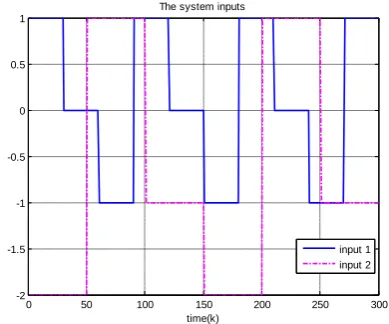
The inputs
u k u1
, 2 k
are a multi-step signal sequence which shown in Fig. 8, and
e k e k1
, 2
are a white noise sequence with zero mean and variance 20.12. The output responses
y k1
,y2 k
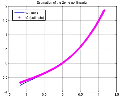
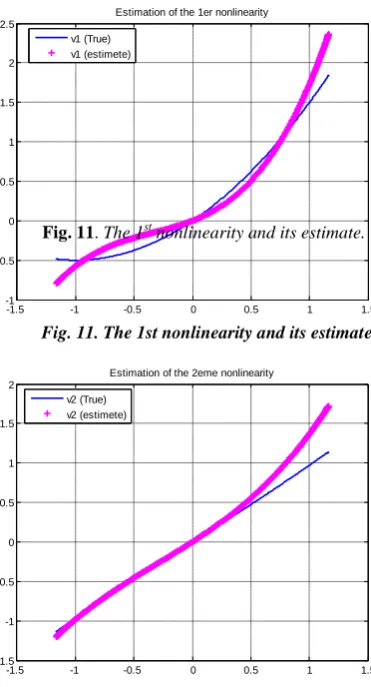
and their estimates are shown in Fig. 9 and 10 respectively. True nonlinearity and mean estimated nonlinearity are shown in Fig. 11 and Fig. 12 respectively.0 50 100 150 200 250 300
-2 -1.5 -1 -0.5 0 0.5 1
The system inputs
time(k)
[image:6.595.331.526.76.238.2]input 1 input 2
Fig. 8. The training input sequence for
u
1
k
andu
2
k
.Fig. 9. The 1st output and its estimate.
[image:6.595.331.523.269.437.2] [image:6.595.47.289.300.369.2]-1.5 -1 -0.5 0 0.5 1 1.5 -1.5
-1 -0.5 0 0.5 1 1.5 2
Estimation of the 2eme nonlinearity v2 (True)
v2 (estimete)
-1.5 -1 -0.5 0 0.5 1 1.5
-1 -0.5 0 0.5 1 1.5 2 2.5
Estimation of the 1er nonlinearity v1 (True)
[image:7.595.73.259.59.403.2]v1 (estimete)
Fig. 11. The 1st nonlinearity and its estimate.
Fig. 11. The 1st nonlinearity and its estimate
Fig. 12. The 2nd nonlinearity and its estimate.
By using the proposed method, the matrices in the ARX model and the vectors of the nonlinearity are converged to the following :
1 2
1 2
0.6861 0.1968 0.1796 0.0987
ˆ ; ˆ ;
0.0995 0.4958 0.1468 0.1373 0.2329 0.0637 0.0455 0.0117
ˆ ; ˆ
0.3861 1.0093 0.0086 0.0243
A A
B B
1 2
ˆ 0.5794 0.5782 ; ˆ 0.9568 0.2183
The results were obtained using the same algorithm that the matrices A kˆ1
, A kˆ2
, B kˆ1
and B kˆ2
are closed to the same matrices in the ARX plant model. In the same way, the output of the system converged to the nonlinearities at the inputs which are shown in Figs. 9, 10, 11 and 12. The different performance criteria with the SVD method between the actual and identified nonlinearities are shown in Table 2.1st system 2nd system
MSE 1.1988 e-005 7.5143 e-007
VAF (%) 100.0000 100.0000
FIT (%) 99.9357 99.9578
Table 2. The different performance criteria
5.3
DISCUSSIONS
In this paper, MIMO Hammerstein model identification based on RLS algorithm and SVD method for decomposition of the linear and nonlinear parameters have been demonstrated for two simulation examples. This approach offers the advantage of being more general than the other approaches to present in other papers such as the LS-SVM approach presented by [13] and JITL approach presented by [11] of made that these two approaches consider that the matrices are selected equal to the identities, on the other hand in our approach we consider the case more general where B is unspecified.
It is important to know the conditions under which the RLS/SVD algorithm will converge. The RLS/SVD is a combination of the RLS and SVD algorithms. Hence, the convergence properties of the RLS/SVD algorithm are directly associated to the convergence properties of the RLS and SVD algorithms. For deterministic systems, it is well known that the RLS produces unbiased estimates of the parameters provided that the process order is known and the input is persistently exciting [23]. On the other hand, the linear model parameters and the static nonlinearity can be obtained simultaneously by solving a set of linear equations followed by the singular value decomposition (SVD). Then, by recurring to SVD and rank reduction, optimal estimates of the parameter matrices characterizing the linear and nonlinear parts can be obtained.
[image:7.595.56.239.489.564.2]Comparing the nonlinearities in Figs. 6 and 7 in the first example and Figs. 11 and 12 in the second example, we can consider that the approach is satisfactory by identifying the nonlinearities. The inputs of the first example are shown in Fig. 3 and that of the second example are shown in Fig. 8. The comparison between real and estimate output curves of the system are given in Figs. 4 and 5 for the first example and Figs. 9 and 10 for the second example.
From Tables 1 and 2 and Figs. 3 to 12, we can infer the following conclusions:
The parameter estimates provided by the identification algorithm converge to their true values.
The responses of the original system and the identified system are very similar.
It is clear that the errors are becoming smaller as k increases. This remark confirms the proposed algorithm. For the same data length, the recursive algorithm gives
good estimated parameters.
The convergence of the estimated parameters to their true values.
The MIMO Hammerstein model outperforms the estimates model for each of the three considered criteria. This state shows that the proposed algorithm is effective.
6.
CONCLUSION
In this paper, we have proposed a new technique for the identification of MIMO Hammerstein ARX systems. The method is based on recursive least squares (RLS) approximation and allows to determine the memoryless static nonlinearity as well as the linear model parameters from a linear set of equations. The obtained estimated parameters of the identification model include the products of the original system parameters. To separate the estimated parameters into the original parameters, the singular value decomposition (SVD) method is discussed. Moreover, the proposed method is applicable to MIMO systems with separate or combined nonlinearities. The recursive algorithm is a novel combination of RLS and SVD algorithms. Simulation results reveal the robustness and effectiveness of the proposed method.
7.
ACKNOWLEDGMENTS
We thank the ministry of higher education and scientific research of Tunisia for funding this work.
8.
REFERENCES
[1] Abonyi, J., Babuska, R., Botto, M.A., Szeifert, F. and Nagy, L., (2000) "Identification and control of nonlinear systems using fuzzy Hammerstein models". Ind Eng Chem Res, 39 pp. 4302 – 4314.
[2] Al-Duwaish, H. and Karim, M.N., (1997) "A new method for the identification of Hammerstein model". Automatica 33 pp. 1871 – 1875.
[3] Bai, E. W., (1998) "An optimal two-stage identification algorithm for Hammerstein–Wiener nonlinear systems". Automatica, 34 (3), pp. 333 – 338.
[4] Bai, E.W., (2004) "Decoupling the linear and nonlinear parts in Hammerstein model identification", Automatica 40 (4) pp. 671 – 676.
[5] Chaoui, F.Z., Giri, F., Rochdi, Y., Haloua, M., and Naitali, A., (2005) "System identification based on Hammerstein model", International Journal of Control 78 (6) pp. 430 – 442.
[6] Ding, F. and Chen, T., (2005) "Identification of Hammerstein nonlinear ARMAX systems", Automatica 41 (9) pp. 1479 – 1489.
[7] Ding, F., Shi, Y. and Chen, T., (2006) "Gradient-based identification methods for Hammerstein nonlinear ARMAX models", Nonlinear Dynamics 45 (1_2) pp. 31 – 43.
[8] Ding, F., Shi, Y. and Chen, T., (2007) "Auxiliary model based least-squares identification methods for Hammerstein output-error systems", Systems & Control Letters 56 (5) pp. 373 – 380.
[9] Ding, F., Chen, T. and Iwai, Z., (2007) "Adaptive digital control of Hammerstein nonlinear systems with limited output sampling", SIAM Journal on Control and Optimization 45 (6) pp. 2257 – 2276.
[10] Ding, F., Peter, L. X., and Liu, G., (2011) "Identification methods for Hammerstein nonlinear systems", Digital Signal Processing 21 pp. 215 – 238.
[11] Hlaing Y.M., Chiu M.-S. and Lakshminarayanan S., (2007) "Modeling and control of multivariable process using generalized Hammerstein model". Chemical Engineering Research and Design Trans, Vol 85 (A4) pp. 445 – 454.
[12] Hua Liang and Bolin Wang, (2007) "Identification of MIMO Hammerstein Models Using Support Vector Machine". ISNN 2007, Part III, LNCS 4493, pp. 399 – 406. Springer-Verlag Berlin Heidelberg.
[13] Ivan Goethals, Kristiaan Pelckmans, Johan A.K. Suykens, Bart De Moor, (2005) "Identification of MIMO Hammerstein models using least squares support vector machines". Automatica 41 pp. 1263 – 1272.
[14] Jia, L., Chiu, M.S. and Ge, S.S., (2005) "Iterative identification of neuro-fuzzy based Hammerstein model with global convergence". Ind Eng Chem Res, 44 pp. 1823 – 1831.
[15] Jia L., Chiu M.S., Ge S.S., (2005) "A noniterative neuro-fuzzy based identification method for Hammerstein processes", Journal of Process Control 15 (7) pp. 749 – 761.
[16] Juan C. Gomez, Enrique Baeyens, (2004) "Identification of block-oriented nonlinear system using orthonormal bases", Journal of Process Control 14 pp. 685 – 697. [17] Jyothi S. N., Chidambaram M., (2000) "Identification of
Hammerstein model for bioreactors with input multiplicities". Bioprocess Engineering 23 pp. 323 – 326 Springer-Verlag.
[18] Kwong Ho Chan, Jie Bao, William J. Whiten, (2006) "Identification of MIMO Hammerstein systems using cardinal spline functions". Journal of Process Control 16 pp. 659 – 670.
[19] Lakshminarayanan, S., Shah, S. L., & Nandakumar, K. (1995) "Identification of Hammerstein models using multivariate statistical tools". Chemical Engineering Science, 50 (22), pp. 3599 – 3613.
[20] Lee, M.W., Huang, H.P. and Jeng, J.C., (2004) "Identification and controller design for nonlinear processes using relay feedback". J Chem Eng Japan, 37 pp. 1194 – 1206.
[21] Lee Y.J., Sung S.W., Park S., (2005) "Input test signal design and parameter estimation method for the Hammerstein–Wiener processes", Industrial and Engineering Chemistry Research 43 (23) pp. 7521 – 7530.
[22] Liu, Y., Sheng, J., and Ding, R., (2010) "Convergence of stochastic gradient estimation algorithm for multivariable ARX-like systems", Computers and Mathematics with Applications 59 pp. 2615 – 2627.
[23] Ljung, L. (1987) "System Identification Theory for the User". Prentice-Hall, Englewood Cliffs, NJ.
[24] Louhichi B., Toumi A., (2008) "Identification of Greenhouse parameters using ARMAX and NARMAX structures", International Review of Physics (I. R. E. PHY.) vol. 2, N. 2, pp. 129 – 138.
[25] Louhichi B., Toumi A., (2010) "Identification of nonlinear Hammerstein – Wiener ARMAX systems", 11th International conference on Sciences and Techniques of Automatic control & computer engineering (STA’10), Monastir, Tunisie.
[27] Pottmann, M., Unbehauen, H. and Seborg, D.E., (1993) "Application of general multimodel approach for identification of highly nonlinear processes". Int J Control, 57 pp. 97 – 120.
[28] Ramos J.A., Durand J.F., (1999) "Identification of nonlinear systems using a B-Splines parametric subspace approach". Proceedings of the American Control Conference, vol. 6, pp. 3955 – 3959.
[29] Sung S.W., (2002) "System identification method for Hammerstein processes". Industrial and Engineering Chemistry Research 41 (17) pp. 4295 – 4302.
[30] Su, H.T. and McAvoy, T.J., (1993) "Integration of multilayer perception networks and linear dynamic models: a Hammerstein modeling approach". Ind Eng Chem Res, 26 pp. 1927 – 1936.
[31] Wang, D.Q. and Ding, F., (2008) "Extended stochastic gradient identification algorithms for Hammerstein – Wiener ARMAX systems", Computers and Mathematics with Applications 56 pp. 3157 – 3164.
[32] Zhu Y., (2000) "Identification of Hammerstein models for control using ASYM", International Journal of Control 73 (18) pp. 1692 – 1702.
9.
AUTHORS PROFILE
Badreddine LOUHICHI was born in Sfax (Tunisia) on
August 1976. He received the Electrical Engineering Diploma from Sfax Engineering National School (ENIS), University of Sfax, Tunisia, in 2001. He prepared in collaboration with the Polytechnique School, University of Nantes, France, his diploma of DEA. He received the DEA (Master) in automatic control from ENIS in 2002. He is currently preparing the Ph.D. in the field of automatic control. He is a member of the Laboratory of Sciences and Techniques of Automatic control & computer engineering (Lab-STA) of the University of Sfax. He is currently an Associate Professor of electric engineering in the Faculty of the Sciences of Sfax, Tunisia.
Ahmed TOUMI was born in Sfax (Tunisia) on November
1952, he is Professor in the Sfax Engineering National School (ENIS), received the Electrical Engineering Diploma from (ENIS/Tunisia), the DEA (Master) in Instrumentation and Measurement from University of Bordeaux-1/France in 1981