Knee Joint Articular Cartilage Segmentation, Visualization and Quantification using Image Processing Techniques: A Review

Knee Joint Articular Cartilage Segmentation,

Visualization and Quantification using Image Processing

Techniques: A Review

M. S. Mallikarjuna Swamy

Research Center, Dept. of Biomedical Engineering Bapuji Institute of Engineering and Technology

Davangere -577004, India

Mallikarjun S. Holi

Research Center, Dept. of Biomedical Engineering Bapuji Institute of Engineering and Technology

Davangere -577004, India

ABSTRACT

Knee is a complex and articulated joint of the body. Cartilage is a smooth hyaline spongy material between the tibia and femur bones of knee joint. Cartilage morphology change is an important biomarker for the progression of osteoarthritis (OA). Magnetic resonance imaging (MRI) is the modality widely used to image the knee joint because of its hazard free and high resolution soft tissue contrast. Cartilage thickness measurement and visualization is useful for early detection and progression of the disease in case of OA affected patients. A wide variety of algorithms are available for knee joint image segmentation. They are classified as pixel based and model based methods. Based on the human intervention required, segmentation methods are also classified as manual, semi-automatic and fully automatic methods. This paper reviews knee joint articular cartilage segmentation methods, visualization, thickness measurement, volume measurement and validation methods.

General Terms

Medical image processing, Computer vision, Pattern recognition

Keywords

Cartilage thickness, MRI, Osteoarthritis, Knee joint, Image segmentation.

1.

INTRODUCTION

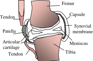
Knee joint is the largest and most complex joint in human body. It is a hinge joint formed by the condyles of the femur, condyles of the tibia and posterior surface of the patella (knee cap). Intra-capsular structure of knee joint includes synovial membrane with synovial cavity filled with synovial fluid, articular cartilage, menisci (semi-lunar cartilages), cruciate ligaments, and burse. Fig.1 shows anatomy of knee joint.

Ligaments, which are extra capsular structures, are the strong band of connective tissue that connects one bone to another across a joint providing strength and stability to the joint. Articular Cartilage is a thin layer of high-quality, ultra-slippery hyaline material which covers the ends of bones which slide against each other at the joint. Articular cartilage covers the patella, tibia and femur in the regions where the bones articulate with one another.

Osteoarthritis (OA) is a most common disease of the knee joint affecting the elderly people. It occurs when cartilage becomes soft and get eroded due continuous wear and tear movements and with ageing. This often leads to inflammation, decrease in motion of joint due to stiffness, and formation of bone spurs (tiny growths of new bone). This decreases the ability of the cartilage to work as a shock-absorber to reduce the impact of stress on the joints. Fig.2 shows OA affected knee joint.

The remaining cartilage wears down faster, and eventually, the cartilage in some regions may disappear altogether, leaving the bones to rub against one another during motion. It is at this stage that bone spurs may form. With OA, synovial fluid does not provide proper lubrication, which leads to pain, inflammation and restriction of movements at the joints. In severe OA there will be complete breakdown of cartilage over a period of time, leading to severe pain and joint loss. There is no artificial material that can replace only the cartilage at the joint.

The OA affects about 21 million people in the United States. By the age 65, the majority of the population has radiographic evidence of OA and 11 percent have symptomatic OA of the Fig.1 Knee joint anatomy

Femur

Tibia Articular

cartilage Meniscus

Patella

Capsule

Synovial membrane Tendon

Tendon

Fig.2 OA affected knee joint

Exposed bone

Eroded cartilage

Bone spurs

knee [1]. According to study [2] conducted on Indian population, OA was present in only 50.2% of the elderly aged 65-74 years, whereas it was 97.7% in elderly aged 84 years and above. Prevalence of OA increased as body mass index (BMI) increased. It was 51.36% amongst elderly with BMI less than 25, whereas it increased to 100% amongst elderly with BMI equal to or more than 40.

2.

BACKGROUND

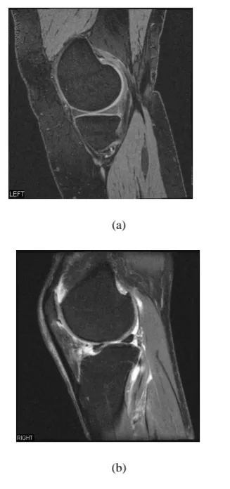
MRI can image cartilage, bone and other surrounding soft tissues distinctly. MRI is a non-invasive and repetitive imaging study of an individual is possible without side effects. The assessment of cartilage dimensions is important for the study of the progression of cartilage damage due to OA. MRI images are widely used for diagnosis of knee joint abnormalities. This imaging modality can be used in in-vivo and in-vitro studies of anatomical structures. MRI provides knee joint images in sagittal, coronal and axial planes. Sagittal images give better view of cartilage than the other two. Fig.3 shows the MR images of knee joints (a) normal (b) OA affected.

(a)

(b)

Fig. 3. MR image of (a) Normal knee joint (b) OA affected knee joint

High resolution gradient echo MRI sequences with fat suppression are the most useful techniques for quantization of cartilage dimensions. Even though, MRI directly visualizes the cartilage for progressive assessments, image processing techniques are needed for better visualization and quantification. Knee joint cartilage thickness measurement gives vital information in the diagnosis and treatment of

progression of OA. The 3D visualization gives complete information and insight on cartilage degradation and menisci tears. In specific cases, MR images with high signal to noise ratio with high resolution are used for in-vitro studies. But in most of the in-vivo, low contrast knee image slices are used. The 3D reconstruction algorithms are used to obtain the data missing in 2D images.

3.

KNEE JOINT SEGMENTATION

METHODS

Image segmentation is defined as portioning of an image into non overlapping constituent regions that are homogeneous with respect to some characteristic such as intensity or texture. A segmentation method finds those set that correspond to distinct anatomical structures or regions of interest in the image [3]. If the domain of the image is given by Ω then the segmentation problem is to determine the sets 𝑆𝑘∁ 𝛺 whose union is the entire domain Ω. Thus the sets that make up segmentation must satisfy

𝛺 = 𝐾𝑘=1𝑆𝑘 (1)

Where𝑆𝑘∩ 𝑆𝑗 = ∅ 𝑓𝑜𝑟 𝑘 ≠ 𝑗 and each 𝑆𝑘 is connected.

Knee joint image segmentation is a very challenging task because of the complexity of joint. Knee joint segmentation methods can be classified into three categories based on manual intervention required, namely manual, semiautomatic and fully automatic. The manual segmentation methods are simple but laborious and time consuming for 3D reconstruction. Semi automatic methods are developed to reduce the manual intervention by automating few steps of processing. Fully automatic methods are also developed with certain limitations. Knee Segmentation methods are also classified into two categories. Pixel or intensity based segmentation methods and model or geometry based segmentation methods. The edge detection, thresholding, region growing and region merging methods are pixel based techniques. On the other side snake algorithms, active contours, atlases and deformable models are geometry based.

3.1

Pixel or Intensity based Segmentation

Methods

In the earlier edge detection method of Kshirsagar et. al. [4], Canny edge detection and template matching techniques are used. To locate the boundary of femur the edge map is cross correlated with standard template. Approximate centre of the femur is obtained. Mask is obtained to delineate the exact boundaries. They extended the method to 3D edge detection for automatic delineation of cartilage from 3D MR images of human knee joint. Canny edge detection technique is used recursively to segment the cartilage [5]. The Canny edge detection operator returns a value for the first derivative in the horizontal direction (Gx) and the vertical direction (Gy). From this the edge gradient and direction can be determined [6].

∇𝑓 𝑥, 𝑦 = _𝜕𝑥 𝜕𝑓 ,𝜕𝑓_𝜕𝑦 (2)

The magnitude (edge strength) of the gradient is then approximated using the formula:

|G| = |Gx| + |Gy| and Θ = tan-1

(Gy/Gx) (3)

Region of interest is obtained from each image as in the manual segmentation by fixing the points along the curves. An interpolated cubic B-spline curve is fitted for the points. The image gradient vector is evaluated using the Prewitt convolution kernel. The B-spline curve, which follows the contour of the desired surface, is then sampled at 0.5 mm intervals.

A B-spline of degree n is derived through n convolutions of the box filter, B0. Thus, B1=B0*B0 denotes a B-spline of degree 1, yielding the familiar triangle filter. The B-spline of degree 1 is equivalent to linear interpolation. The second degree B-spline B2 is produced by convolving B0*B1. The cubic B-spline B3 is generated from convolving B0*B2. That is B3=B0*B0*B0*B0 [8]. The filter function is

𝑕 𝑥 =1

6

3 𝑥 − 6 𝑥 + 4 0 ≤ 𝑥 < 1 − x|3_{+ 6 x|}2_{− 12 x + 8 1 ≤ |x| < 2}

0 2 ≤ 𝑥

(4)

Cashman et al. [9], developed algorithm, in addition to edge detection techniques, thresholding is performed to exclude all pixels below one half of the average intensity of the image. Boundary discontinuities are bridged using B-spline interpolation. Selecting a seed point inside the bone and using a recursive region growing procedure the interior of the bone is filled and labeled. A morphologically dilated copy of the bone boundary is applied as a mask to the raw MR image. The bone region is subtracted to leave a shell of cartilage. In radial search method developed by Poh and Kitney [10], an origin is fixed at center of femur and horizontal line is drawn. Each vector of radius R and angle θ with horizontal line is defined. Pixel intensities and coordinates along the line of radius R are taken. A threshold method is used to detect the inner boundaries. The coordinates of pixel at which intensity crosses the threshold value is stored. Similarly a vector in the reverse direction is used to detect the outer boundary. The search for outer boundary starts at distance w away from the inner boundary and in the direction towards the origin. If the pixel intensities are greater than the threshold the coordinates of the outer boundary are saved. This procedure is repeated for 0-180 degree to cover the entire cartilage. B-spline curve is used to get continuous contour. Segmented images are obtained by masking the original image with this contour. In the method developed by Gamio et al. [11] Bezier splines are used. The control points are placed inside the cartilage following its shape to create a Bezier spline. Rays perpendicular to the spline on the control points are traced to find the bone cartilage interface. The edges are found based on the first derivative of brightness using bicubic interpolation along the line profiles. A graph-cut method developed by Shim et al. [12] seeds are placed manually (curvilinear marks) over specific anatomic regions. The seeds are propagated to neighboring pixels and then segmented. The method is compared with manual method. In another algorithm of Gamio et al. [13], the cartilage edges are enhanced using the anisotropic diffusion algorithm. Edges are detected after filtering the image with a Laplacian of Gaussian (LOG) filter. The position of the control points of the Bezier splines is then automatically adjusted to overlap the closest edges. Unsatisfactory control points are adjusted manually to segment the cartilage. Lee and Chung [14] utilized the moment preserved thresholding to estimate the region of interest (ROI). An ROI based wavelet enhancement is used to restrict the contrast improvement only around the bone edges. A new approach called Filled Laplacian of Gaussian (FLOG)

converts the edge detection results using LOG into a region based format through the flow fill operation. The MR images are resampled in the neighborhood of the bone surface. Texture-analysis technique is used by Dodin et al. [15], segmentation is optimized by filtering, the cartilage is discriminated as a bright and homogeneous tissue. This process of excluding soft tissues enables the detection of the external boundary of the cartilage. A technology based on a Bayesian decision criterion enables the automatic separation of the cartilage and synovial fluid. In radial transformation method developed by Chang et al. [16] the original image is resampled in a radial approach to form a new image, called radial image. The cartilage boundaries are first delineated on the radial image in a row by row fashion, which simplifies the two dimensional segmentation to a one dimensional. The pixels of delineated boundaries are then transformed back to the original image space by simple coordinate computation. After further modification and thinning procedures, the final segmentation results are obtained in the original image space. In watershed based algorithm of Ghosh et al. [17], the procedure is initiated by sorting the pixels into a simple array according to intensity, and assigning a threshold pixel value. The cartilage contour is detected automatically by selecting contours with maximum perimeter and minimum cluster label. Improved watershed algorithm is developed by Grau et al. [18] for cartilage segmentation. This method combines watershed algorithm with atlas registration. This utilizes the prior information based on calculation. The method overcomes the limitations of watershed segmentation method like over segmentation, poor detection of low signal to noise ratio structures and thin boundaries. A fully automatic method using voxel classification is developed by Folkesson et al. [19]. The algorithm is based on kNN classifier to reduce processing time. The basic idea behind this algorithm is not to classify all voxels but to focus mainly on the cartilage voxels. If a voxel is classified as cartilage, it continues with classification of the neighboring voxels and this expansion process continues until no more cartilage voxels are found. The method also works with low field MRI data.

3.2

Shape or Model based Methods

In these methods, segmentation is based on cartilage shape or model developed. The development of the cartilage model is based on prior knowledge obtained for a group of population under study. Model is registered on the MR image cartilage. These registered active contours are deformed to match the cartilage of the image. The deformed contour is used as cartilage map [20]. Snakes or active contours are energy minimizing curves that deform under the influence of internal forces within curve itself and external force derived from the image to minimize the energy function. The snake is defined parametrically as v(s) =[x(s), y(s)], where x(s), y(s) are x, y coordinates along the contour and s Є [0, 1]. The energy function to be minimized is

𝐸𝑠𝑛𝑎𝑘𝑒 = 𝐸₀1 𝑠𝑛𝑎𝑘𝑒 𝑣 𝑠 𝑑𝑠 (5)

= (₀1 𝐸𝑖𝑛𝑡 𝑣 𝑠 + 𝐸𝑖𝑚𝑎𝑔𝑒 𝑣 𝑠 + 𝐸𝑐𝑜𝑛 𝑣 𝑠 )𝑑𝑠 (6)

Where Eint represents the internal energy of the spline due to

bending, Eimage denotes image forces, and Econ external

constraint forces [21].

coordinate system (LCS) is developed for the femoral and tibial cartilage boundaries that provide a standardized representation of cartilage geometry, thickness, and volume. The LCS can be registered in different data sets from the same patient so that results can be directly compared. Cartilage boundaries are segmented from 3D MRI and transformed into offset maps, defined by the LCS. Gaps in the offset map resulting from inter slice distance are filled using a bi-cubic interpolation scheme. A method for model based segmentation of 3D MRI scans of the human knee is presented by Kapur et al. [24]. A probabilistic model describing the spatial relationships between features of the human knee is constructed from 3D manually segmented data. In conjunction with feature detection techniques this model is used to segment knee MRI scans in a Bayesian framework. A Diffusion Snake segmentation algorithm is performed on synthetic and real MR images of articular cartilage by Tejos et al. [20]. The Diffusion Snake algorithm comprises two procedures: training and segmentation. A set of images are used to train the software about the shape and allowable shape variations in the feature chosen for segmentation. The training process involves manual land-marking with an identical number of equally-spaced landmarks for each data set. The algorithm proved to be robust to missing boundaries and the initial contour converges over large distances. A method based on directional gradient vector flow snakes is developed by Tang et al. [25]. To overcome the limitations of snake based methods gradient based snakes are proposed. Using external force, the traditional GVF snake may be attracted to strong edges that have the opposite gradient direction with respect to the intended boundary. The GVF snake is more stable and converges to the correct surfaces. In the Method developed by Tameem et al. [26] based on the creation of morphological atlases of the cartilage using normal subjects segregated by age, sex, and gender. Active shape models are used to represent the variance in cartilage shape within a given population. These atlases capture the variation of shape in normal subjects and are then used to classify „normal (asymptomatic of OA)‟ or „abnormal (symptomatic of OA)‟. In the 3D statistical shape model (SSM) based method of segmentation developed by Fripp et al. [27] SSM of the bones is used to represent the variability in shape of the bones. The atlas used is an arbitrary case from the database. The surface associated with the atlas is propagated to the image using the obtained affine transform (T), and its pose and shape parameters are estimated. These parameters are then used to initialize the Active shape models (ASM) segmentation. The ASM segmentation consists of two components: a SSM and matching criteria. The segmentation is performed with two steps which are repeated until convergence. In the first step called deformation, in this position of each point is moved in 3D to the best nearby match, in this case along a profile normal to the surface. Second step called shape restriction: the pose and shape parameters of the deformed surface are estimated using the SSM. Adaptive external forces are used to the 3-D smoothing B-Spline active surface (SBAS) in a method proposed by Xian et al. [28]. This improves the accuracy and robustness of cartilage segmentation. For each MRI data, the initial snake for bone cartilage interface will be the same which is set according to the shape and position of the segmentation target. The central points of the volume data are assumed to be identical. Secondly, adaptive external forces, which incorporate the relationship between the evolution process and external force range, govern snake evolution. A fast global minimization snake model is developed by Tran et al. [29]. This is a new segmentation method based on the Chan–Vese (C-V) model to determine

the global minimization of standard geometric active contour (GAC) is considered. This model is not based on the image gradient such as classical snake model detecting the boundaries of the object, but on the homogeneous regions. This fast global minimization of snake model is used to segment the MRI Image. This method overcomes the existence local minimum in energy function, increase the convergence of the segmentation process and reducing time need to converge. Active Appearance Models (AAMs) developed by Williams et al. [30] are extensions of Statistical Shape Models (SSMs) which, in addition to information on an object‟s shape, contain information on its appearance. The appearance of the objects is captured as a set of samples of the image around each corresponding point. To enable automatic segmentation of the bone, the AAM uses the training set to learn the relationship between perturbations of the parameters (pose, scale and combined shape and texture) and deviation from the required solutions. Thus, given a new image, not part of the training set, and an approximate initialization, it is able to determine how to alter the pose and combined shape and texture parameters in a way which moves and morphs the bone shape until the best fit of the model is found within the image. A method for simultaneous segmentation of multiple interacting surfaces belonging to multiple interacting objects, called LOGISMOS (layered optimal graph image segmentation of multiple objects and surfaces), is developed by Yin et al.[31]. The approach is based on the algorithmic incorporation of multiple spatial inter-relationships in a single n-dimensional graph, followed by graph optimization that yields a globally optimal solution. For the knee joint segmentation results found are robust and accurate.

4.

QUANTIFICATION OF CARTILAGE

THICKNESS AND VOLUME

The thickness of a cartilage layer is defined as the Euclidian distance between the bone-cartilage interface and the cartilage-synovium interface [26]. Thickness measurements are made from the inner cartilage boundary in a direction normal to the inner boundary toward the outer cartilage boundary. The Euclidian distance 𝐷𝐸 between a point p belonging to the outer boundary of the cartilage and the nearest point r belonging to the inner boundary I is computed [29] using

𝐷𝐸 𝑝 = 𝑚𝑖𝑛 𝑝𝑥− 𝑟𝑥 2+ 𝑝𝑦− 𝑟𝑦 2

+ 𝑝𝑥− 𝑟𝑧 2

𝑟 ∈ 𝐼 (7)

thickness. In the 2D active contour method of Kauffman et al. [23] thickness and volume are computed using offset maps. The cartilage thickness is computed by iteratively searching along the 3D inner-surface normal starting from the inner boundary offset map and proceeding until the outer-surface offset-map value is reached. Repeating the process for every point in the inner-surface generates a thickness-map that represents the local thickness at every location on the bone surface. Finally total volume is computed adding the local volumes. Total volume 𝑉𝛺 of articular cartilage is computed using local volumes𝑉𝑖,𝑗 obtained [23].

𝑉𝛺= 𝑉𝑖𝑗 ∀ 𝑉𝑖,𝑗 ∈ 𝛺 (8)

In the technique developed by Mlejnek et al. [32], cartilage visualized by unfolding of the cartilage and depicting it as a height field. The height field representation of the cartilage eliminates the complexity of the 3D shape of the cartilage. The user can directly inspect the cartilage thickness. In another work carried out by Gamio et al. [11], the thickness is measured for three different cases: cartilage with no shape interpolation (anisotropic resolution), cartilage with shape interpolation using distance fields, and cartilage with shape interpolation using the morphing technique. The cartilage volume is also computed for the same three cases and it is done with two different methods: counting the number of voxels inside and on the cartilage contours; and counting the same voxels with different weighting according to predefined patterns of voxels. In the method suggested by Folkesson et al. [19], the normal at each point on the bone interface surface is determined by a local surface fitting technique. The cartilage thickness is then calculated as the distance between the points of intersection of the normal to the two interfaces. The cartilage volume is calculated by voxel count for each femoral and tibial compartment. The values for mean and maximal thickness and volume for the cartilage are assessed separately for the medial and lateral tibial and femoral plateaus. The thickness values at each point are represented by a color map by Poh et al.[33] For visualization the thickness values are plotted as a contour plot in terms of their angular and slice position to outline the 2D shape of the cartilage.

5.

STATISTICAL ANALYSIS AND

VALIDATION

The measurement of cartilage thickness is reproducible, when the method used for segmentation is objective. Manual delineation of cartilage results in poor inter and intra- observer reproducibility. To determine the precision of the MRI based cartilage measurements the root-mean square average (RMS thickness), standard deviation (SD) and coefficient of variation (CV) of mean thickness are determined from the repeated image data sets [7]. The CV is computed as

𝐶𝑉 = 100 ∗ _{𝐴𝑣𝑒𝑟𝑎𝑔𝑒}𝑆𝐷 (9)

The SD and CV over mean value of the thickness and volume measurements from the repeated MR examinations indicates the measure for assessing the reproducibility [34]. The reproducibility of the two segmentation methods is determined with the dice similarity coefficient (DSC), which is a measure of how closely two independently segmented cartilages match when one is superimposed on the other[15]. The DSC is computed as

𝐷𝑆𝐶 𝑂1, 𝑂2 = _{𝑛 𝑂}𝑛(𝑂1∩𝑂2)

1 +𝑛 𝑂2 /2=

𝑉𝑜

𝑉𝑚 (10)

Where 𝑂1and 𝑂2 are segmented images, Vo is the overlapped

volume and Vm is the mean volume. The DSC ranges from 0

for no overlap to 1 for perfect agreement between segmented cartilage volumes. Kshirsagar et al. assessed the reproducibility of the method by MR scanning the healthy volunteers repeatedly at different times [4]. In vitro and in vivo study of Cohen et al. [7] cadaveric knees is imaged using MRI and Stereophotogrammetric (SPG) methods. Later cadaveric knees are bisected to measure actual cartilage thickness. This study assessed the 3D accuracy of MRI for measuring articular surface topographies and cartilage thicknesses of human cadaveric knee joints in comparison with the calibrated SPG method. The overall thickness accuracy for the surface is computed as the RMS residual expression

𝑅𝑀𝑆 = 𝑡𝑖

𝑚𝑟𝑖_−𝑡 𝑖𝑠𝑝𝑔

2

𝑛 𝑖

1 2

(11)

Where n is the number of sampled points. Cartilage thickness obtained from MR images is compared with the thickness obtained from SPG images. In an automated technique [9], for validation bovine and porcine cadaveric knees are given artificial cartilage lesions and then imaged. The animal validations showed close agreement between direct lesion measurements and those obtained from the MR images. The accuracy of the automated behavior of the method Kaufmann et al. [23] is assessed, using realistic, synthetic 3D MR images of a human knee. The cartilages of 16 porcine knees are scraped off and its volume is measured using a saline displacement method after image acquisition [11]. The four image data sets for each of the four specimens for the individual tibia and talar cartilage layers are considered by Tang et al. for computation of RMS thickness, SD and CV [25]. Poh and Kitney [34] conducted inter observer and intra observer study. In this each of the patient data sets are segmented by a single observer four times using the semi-automatic segmentation method. In order to focus on the effect of intra-observer variability, the same dataset is not segmented consecutively on the same day. This reduced the use of prior knowledge obtained during the segmentation of the same dataset. The method of Folkesson et al.[19] is compared with manual segmentation. The results are found matching with manual method. The manual and semi-automated segmentation methods are evaluated by Shim et al.[12]. Methods are compared for efficiency and inter-observer and inter-method reproducibility. Efficiency is determined according to segmentation processing time. The DSC and CV are determined for repeated cartilage segmented volume measurements. In the texture analysis technique of Dodin et al. [15], the validation is done in two studies. In the first study nine knee OA patients are included, a comparison of the cartilage volume and changes over time between the developed automatic system and a validated semi-automatic cartilage volume system are compared. In the second study five knee OA patients are included; the measurement error of the method is evaluated with a test-retest analysis.

6.

DISCUSSION

classification algorithm [19] and statistical shape model [30]. All these methods delineate cartilage boundaries in two or three-dimensional image spaces.

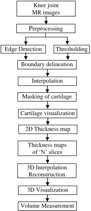
Manual methods consume more time. Semi-automatic methods take less time. The amount of manual intervention decides the reproducibility of the results. However statistical methods are indicative for the reproducibility of the results. Pixel or intensity based techniques involve simple procedures. Model based methods involve advanced procedures of image segmentation. The steps of cartilage segmentation, thickness measurement and 3D visualization are summarized as in the earlier studies [35] and shown in Fig.3.

Obtained MR images are preprocessed for type conversion, noise removal. Edge detection is technique like canny or Prewitt detects the boundaries of the femur, tibia and cartilage. Thresholding is performed on the images to exclude pixels whose intensity are less than the half the average intensity of the image. Missing boundaries can be obtained manually. The boundaries are re-sampled and interpolated. The B-spline interpolation technique can be used. The image can be masked to separate the cartilage. The method is further extended for 3D cartilage visualization and volume measurement. The thickness maps of cartilage obtained after processing individual slices are stored. The cartilage thickness in between the slices is obtained by 3D interpolation. Volume is computed by adding the number of voxels in the visualized cartilage. The cartilage extracted from knee MRI using this method is visualized in 3D and shown in Fig. 4.

Fig.4 Visualized knee cartilage in 3D

The procedure of segmentation and thickness measurement can be repeated several times to ensure the repeatability of the method. Then on each measurement point the thickness readings are averaged.

7.

CONCLUSION

The different segmentation methods of knee joint cartilage are discussed. Manual techniques have drawbacks of inter user reproducibly and intra user reproducibility of measurements. Semi automatic and automatic techniques are used to overcome these difficulties. Model based segmentation techniques are also discussed. Methods adopted for thickness measurement in 2D, visualization in 3D is also envisaged. Finally statistical measures adopted for accuracy, precision, efficiency of measurements and validation methods are discussed. Manual methods are time consuming and semi automatic methods have the problem of reproducibility. Fully automatic methods are complex image processing techniques and few of them need prior knowledge of knee images under study. Combined methods of intensity and model based techniques are also developed. There is still scope to develop a method which is efficient in time and computational complexity for segmentation, visualization and better quantification.

8.

ACKNOWLEDGMENTS

Osteoarthritis Initiative (OAI), National Institute of Health, USA for providing knee MR Images.

9.

REFERENCES

[1] Samson DJ, Grant MD, Ratko TA, Bonnell CJ, Ziegler KM and Aronson N. “Treatment of primary and secondary osteoarthritis of the knee”, Evidence Report, AHRQ Publication, Technology Assessment No. 157, No. 07-E012. September 2007.

[2] Sharma MK, Swami HM, Bhatia V, Verma A, Bhatia S, and Kaur G., “An epidemiological study of correlates of osteo-arthritis in geriatric population of UT Chandigarh”, Indian Journal of Community Medicine, vol 32, pp.77-8, 2007.

[3] Dzung L. Pham, Chenyang Xu, and Jerry L. Prince, “Current methods in medical image segmentation”, Annual Review of Biomedical Engineering, vol. 02, pp. 315–37, 2000

[4] Kshirsagar, M.D. Robson, P.J. Watson, N.J. Herrod, J.A. Tyler and L.D. Hall, “Computer analysis of MR images of human knee joints to measure femoral cartilage thickness”, Proc. of 18th Annual Int. Conf. IEEE

Cartilage visualization

P

Thresholding

Interpolation

Masking of cartilage

2D Thickness map Knee joint MR images

Edge Detection

Boundary delineation

Fig.3. Thickness and volume measurement of knee cartilage

Thickness maps of „N‟ slices

3D Interpolation Reconstruction

Engineering in Medicine and Biology, Amsterdam, 1996, pp. 746-747.

[5] Kshirsagar, P.J. Watson, N.J. Herrod, J.A. Tyler, and L.D. Hall, “Quantification of articular cartilage dimensions by computer analysis of 3D MR images of human knee joints”, Proc.19th Int. Conf. IEEE EMBS, Chicago, IL. USA, 1997, pp. 753-756

[6] John Canny, “A Computational Approach to Edge Detection”, IEEE Trans. On Pattern Analysis and Machine Intelligence, Vol. 8, No. 6, pp 679-698, 1986.

[7] Zohara A. Cohen, Denise M. Mccarthy, S. Daniel Kwak, Perrine Legrand, Fabian Fogarasi, Edward J. Ciaccio And Gerard A. Ateshian, “Knee cartilage topography, thickness, and contact areas from MRI: in-vitro calibration and in-vivo measurements”, Osteoarthritis and Cartilage, vol. 7, pp. 95–109, 1999.

[8] Póth Miklós, “Comparison of convolutional based interpolation techniques in digital image processing”, Proc.of 5th _{International Symposium on Intelligent}

Systems and Informatics, July 24-25, 2007, Subotica, Serbia, pp 87-90.

[9] Peter M. M. Cashman, Richard I. Kitney, Munir A. Gariba, and Mary E. Carter, “Automated techniques for visualization and mapping of articular cartilage in MR images of the osteoarthritic knee: a base technique for the assessment of microdamage and submicro damage”, IEEE Trans. on Nanobioscience, vol. 1, no. 1, pp. 42-51, 2002.

[10] C. L. Poh and R. I. Kitney, “Viewing interfaces for segmentation and measurement results”, Proc. 27th Annual Conf. IEEE Engineering in Medicine and Biology, Shanghai, China, 2005, pp. 5132-5135.

[11] Julio Carballido-Gamio, Jan S. Bauer1, Keh-Yang Lee, Stefanie Krause, and Sharmila Majumdar, “Combined image processing techniques for characterization of MRI cartilage of the knee”, Proc. 27th Annual Conf. IEEE Engineering in Medicine and Biology, Shanghai, China, 2005 , pp. 3043-3046.

[12] Hackjoon Shim, Samuel Chang,Cheng Tao,Jin-Hong Wang,C. Kent Kwoh, and Kyongtae T. Bae, “Knee cartilage: efficient and reproducible segmentation on high- spatial-resolution MR images with the semiautomated graph-cut algorithm method1”, Radiology, vol. 251, no. 2, pp. 548-556, 2009.

[13] J. Carballido-Gamio, K. Lee1, E. Ozhinsky, S. Majumdar, “MRI cartilage of the knee: segmentation, analysis, and visualization”, Proc. Intl. Soc. Mag. Reson. Med. 2004, p-210.

[14] Jiann-Shu Lee and yi-Nung Chung, “Integrating edge detection and thresholding approaches to segmenting femora and patellae from magnetic resonance images”, Biomedical Engineering Applications, Basis & Communications, vol. 17, no.1, pp. 1-11, 2005.

[15] Pierre Dodin, Jean-Pierre Pelletier, Johanne Martel-Pelletier, and François Abram, “Automatic human knee cartilage segmentation from 3D magnetic resonance images”, IEEE Trans. on Biomedical Engineering, vol. 57, no. 11, pp. 2699-2711, 2010.

[16] Ku-Yaw Chang, Shao-Jer Chen, Lih-Shyang Chen, and Cheng-Jung Wu, “Articular cartilage segmentation based

on radial transformation”, Proc. of 9th International Conf. on Hybrid Intelligent Systems 2009, pp. 239-242.

[17] Srinka Ghosh, Olivier BeufL, Michael Ries , Nancy E. Lane, Lynne S Steinbach, Thomas M. Link, and Sharmila Majumdar, “Watershed segmentation of high resolution magnetic resonance images of articular cartilage of the knee”, Proc. of the 22nd Int. Conf. Annual EMBS, 2000, pp. 3174-3176.

[18] V. Grau, A. U. J. Mewes, M. Alcañiz, R. Kikinis, and S. K. Warfield, “Improved watershed transform for medical image segmentation using prior information”, IEEE Trans. on Medical Imaging, vol. 23, no. 4, pp. 447-458, 2004.

[19] Jenny Folkesson, Erik B. Dam, Ole F. Olsen, Paola C. Pettersen, and Claus Christiansen, “Segmenting articular cartilage automatically using a voxel classification approach”, IEEE Trans. on Medical Imaging, vol. 26, no. 1, pp.106-115, 2007.

[20] Cristián Tejos, Laurance D. Hall, and Arturo Cárdenas-Blanco, “Segmentation of articular cartilage using active contours and prior knowledge”, Proc. of the 26th Annual Int. Conf. of the IEEE EMBS, San Francisco, CA, USA , 2004, pp. 1648-1651.

[21] Sonka, Hlavac and Boyle, “Digital image processing and computer vision”, Cenage Learning, 2008.

[22] Thi-Thao Tran, Po-Lei Lee, Van-Truong Pham and Kuo-Kai Shyu, “MRI Image segmentation based on fast global minimization of snake model”, Proc. of 10th Intl. Conf. on Control, Automation, Robotics and Vision, Hanoi, Vietnam, 2008, pp. 1769-1772.

[23] Claude Kauffmann, Pierre Gravel, Benoît Godbout, Alain Gravel, Gilles Beaudoin, Jean-Pierre Raynauld, Johanne Martel-Pelletier, Jean-Pierre Pelletier, and Jacques A. de Guise, “Computer-aided method for quantification of cartilage thickness and volume changes using MRI: validation study using a synthetic model”, IEEE Trans. on Biomedical Engineering, vol. 50, no. 8, pp. 978-988, 2003.

[24] Tina Kapur, Paul A. Beardsley, Sarah F. Gibson, W. Eric L. Grimson, and William M. Wells, “Model based segmentation of clinical knee MRI”, Proc. of the 6th Int. Conf. on Computer Vision (ICCV-98), Bombay, India, 1998.

[25] Jinshan Tang, Steven Millington, Scott T. Acton, Jeff Crandall, and Shepard Hurwitz, “Surface extraction and thickness measurement of the articular cartilage from MR images using directional gradient vector flow snakes”, IEEE Trans. on Biomedical Engineering, vol. 53, no. 5, pp. 896-907, 2006.

[26] Hussain Z. Tameem, Luis E. Selva, and Usha S. Sinha, “Morphological atlases of knee cartilage: shape indices to analyze cartilage degradation in osteoarthritic and non-osteoarthritic population”, Proc. of 29th Annual Int. Conf. of the IEEE EMBS, Cité Internationale, Lyon, France, 2007, pp. 1310-1313.

[28] Xian Du, Jérôme Velut, Radu Bolbos, Olivier Beuf, Christophe Odet and Hugues Benoit-Cattin, “3-D Knee cartilage segmentation using a smoothing B-spline active surface”, Proc. of 15th Int. Conf. on Image Processing, 2008, pp. 2924-2927.

[29] Thi-Thao Tran, Po-Lei Lee, Van-Truong Pham and Kuo-Kai Shyu, “MRI Image segmentation based on fast global minimization of snake model”, Proc. of 10th Intl. Conf. on Control, Automation, Robotics and Vision, Hanoi, Vietnam, 2008, pp. 1769-1772.

[30] Tomos G. Williams, Andrew P. Holmes, John C. Waterton, Rose A. Maciewicz, Charles E. Hutchinson, Robert J. Moots, Anthony F. P. Nash, and Chris J. Taylor, “Anatomically corresponded regional analysis of cartilage in asymptomatic and osteoarthritic knees by statistical shape modelling of the bone”, IEEE Trans. on Medical Imaging, vol 29, no.8, pp. 1541-1559, 2010.

[31] Yin Yin, Xiangmin Zhang, Rachel Williams, Xiaodong Wu, Donald D. Anderson, and Milan Sonka, “LOGISMOS-Layered Optimal Graph Image

Segmentation of Multiple Objects and Surfaces: Cartilage segmentation in the knee joint”, IEEE Trans. on Medical Imaging, vol. 29, no. 12, pp. 2023-2037, 2010.

[32] Matej Mlejnek, Anna Vilanova, and Meister Eduard Gr¨oller, “Interactive thickness visualization of articular cartilage”, IEEE Proc. Visualization 2004, pp 521-527.

[33] Chueh-Loo Poh, Richard I. Kitney, “Web-based multilayer viewing interface for knee cartilage”, IEEE Trans. on Information Technology in Biomedicine, vol. 13, no. 4, pp. 546-553, 2009.

[34] C.-L. Poh and R. I. Kitney, “Cartilage thickness visualization using 2D wearmaps and trackback”, Proc. 29th Annual Int. Conf. of the IEEE EMBS, Cité Internationale, Lyon, France, 2007, pp. 2883-2886.