Developing a Computational Model for Pricing Index Future

(1)

Developing a Computational Model for Pricing

Index Future

Shom Prasad Das

Department of Computer Science & Engineering & Information Technology National Institute of Science &

Technology, Palur Hills, Berhampur

Prabhat Kumar Tripathy

Upendra Kumar Panda

ABSTRACT

Forecasting in financial market has been difficult task due to its non linearity and high volatility. Effective modeling of forecasting is a major concern for financial market participants. Artificial Neural Network (ANN) is a statistical technique under the non linear regression model. ANNs do consider the non parametric aspects like semantics, emotions for the calculation of volatilities. A Support Vector Machines (SVM) is a concept in statistics and computer science for a set of related supervised learning methods that analyze data and recognize patterns, used for classification and regression analysis SVMs are a very specific type of learning algorithms that uses the kernel functions. Training SVMs is equivalent to solving a linearly constrained quadratic programming problem so that the solution of SVMs is always unique and globally optimal.In this paper, we have focused on some techniques of soft computing such as Neural Network and Support Vector Machines to predict the future pricing. At last we have compared the output of these two models and found which model gives the optimal solution. This computational model can be widely used to find out the future volatility of share in share market.

General Terms

Your general terms must be any term which can be used for general classification of the submitted material such as Pattern Recognition, Security, Algorithms et. al.

Keywords

Volatility, Financial Time Series Forecasting, Artificial Neural Network, Support Vector Machines.

1. INTRODUCTION

In everyday language, volatility refers to the fluctuations observed in some phenomenon over time. Within economics, it is used slightly more formally to describe the variability of the random (unforeseen) component of a time series. More precisely in financial economics, volatility is often defined as the (instantaneous) standard deviation (or “sigma”) of the random Wiener-driven component in a continuous-time diffusion model.

It is, however, in many situations useful - and indeed standard practice - to formulate the underlying model directly in discrete time, and we shall consider both approaches. Formally, there is also no necessary contradiction between the two strategies, as it is always, in principle, possible to deduce

the distributional implications for a price series observed only discretely from an underlying continuous-time model. At the same time, formulation and estimation of empirically realistic continuous-time models often presents formidable challenges. Thus, even though many of the popular discrete-time models in current use are not formally consistent with an underlying continuous-time price process, they are typically much easier to deal with from an inferential perspective, and as such, discrete-time models and forecasting procedures remain the method of choice in most practical applications.

Rest of the paper is organized as follows. Section 2 gives a brief overview of the two machine learning techniques used in our research. In Section 3 some related works are presented followed by data collection and pre processing techniques in section 4. Section 5 discusses the proposed implementation and in Section 6 experimental results are discussed. Section 7 focuses on conclusion of the research.

2. OVERVIEW OF ANN AND SVM FOR

REGRESSION

Back propagation neural network (BPN) is typical network consisting of set of sensory units that constitute the input layer, one or more hidden layers of computation nodes and an output node. All the neurons of one layer are fully interconnected with all neurons of its just preceding and just succeeding layers. These neural networks are also referred to as multilayer perceptrons (MLPs). BPN are applied to solve some difficult diverse problems by training them in a supervised manner with a highly popular algorithm known as error back-propagation algorithm. This algorithm is based on error correction learning rule. Basically the error propagation algorithm consists of two passes: a forward pass and a backward pass. In forward pass the input vector is applied at the nodes of the network and effect propagates through the network layer by layer and finally output is produced as the actual response of the system. The synaptic weight during the forward pass process is fixed but during the backward pass the synaptic weights are adjusted in accordance with an error correction rule. The error signal is transmitted backward through the network. Hence the network is called as the back propagation neural network.

(2)

that the margin of separation between two classes is maximized. The main objective is to do better classification. Apart from classification, SVM is also used for regression problem. Compared to other neural network regression, SVM has three distinct characteristics when it is used to estimate the regression function. First, SVM estimates the regression using a set of linear functions that are defined in a high-dimensional feature space. Second, SVM carries out the regression estimation by risk minimization, where the risk is measured using Vapnik’s ɛ-insensitive loss function. Third, SVM implements the Structural Risk Minimization (SRM) principle which minimizes the risk function consisting of the empirical error and a regularized term. The study concluded that SVMs provide a promising alternative to the financial time series forecasting. And the strengths of SVMs regression are coming from following point: 1) usage of STRUCTURAL RISK MINIMIZATION; 2) few controlling parameters; 3) global unique solution derived from a quadratic programming. 4) a principled approach to classiﬁcation, regression or novelty detection tasks. 5) SVMs exhibit good generalization. 6) Hypothesis has an explicit dependence on the data (via the support vectors). Hence, it can readily interpret the model.

3. RELATED WORK

Previously various works have been done to compare between the artificial neural network and support vector machines. The feasibility of applying SVM in financial forecasting is first examined by comparing it with the multilayer back-propagation (BP) neural network and the regularized radial basis function (RBF) neural network [1]. The variability in performance of SVM with respect to the free parameters is investigated experimentally. Adaptive parameters are then proposed by incorporating the non-stationary of financial time series into SVM. The objective of some previous studies are based on a MLP is used to determine the relationship between some variables as independent factors and the return of the indices as a dependent element [2]. The different GARCH models have been compared with each other and finally which model provides better volatility is tested. A solution is proposed in order to enhance the forecasting ability of model; there was a transformation of original closing prices into relative difference in percentage of price (RDP) [3]. As mentioned there are four advantages in applying this transformation. The most prominent advantage is that the distribution of the transformed data will become more symmetrical and will follow more closely a normal distribution. This modification to the data distribution will improve the predictive power of the neural network.

Two hybrid models are proposed based on EGARCH and Artificial Neural Networks to forecast the volatility of S&P 500 Index [4]. The estimates of volatility obtained by an EGARCH model are feed forward to a Neural Network. The input to the first hybrid model is complemented by historical values of other explanatory variables. The second hybrid model takes as inputs both series of the simulated data and explanatory variables. The forecasts obtained by each of those hybrid models have been compared with those of EGARCH model in terms of closeness to the realized volatility. The computational results demonstrate that the second hybrid model provides better volatility forecasts. During the past decades, many researchers have predicted stock market returns using artiﬁcial intelligence (AI) approaches. Recently, artiﬁcial neural networks (ANNs) combined with other approaches have been applied to this area. Neural network, dynamic time windows, and case based reasoning (CBR) had

percentage prediction accuracy for stock buying or selling decisions was promising. A novel model was proposed by evolving partially connected neural networks (EPCNNs) to predict the stock price trend using technical indicators as inputs. In order to improve the expressive ability of neural networks, EPCNN utilizes random connection between neurons and more hidden layers to learn the knowledge stored within the historic time series data. As mentioned earlier, previous studies tried to optimize the controlling parameters of ANN using local search algorithms whereas this paper combines global search algorithms with a partially connected neural network to forecast stock price index trend. Previously it is attempted at analyzing the usefulness of artificial neural network for forecasting financial data series with use of different algorithms such as back propagation, radial basis function etc. With their ability of adapting non-linear and chaotic patterns, ANN is the current technique being used which offers the ability of predicting financial data more accurately [6]. "A X-Y-1 network topology is adopted because of X input variables in which variable Y was determined by the number of hidden neurons during network selection with single output." Both X and Y were changed and results were compared.

3.1 DATA SET COLLECTION AND

PREPROCESSING

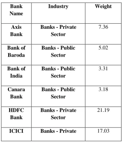
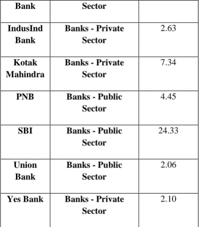
[image:2.595.327.529.529.765.2]

The data for daily closing prices of BANK NIFTY is selected over the time period of 03/11/1995 up to 12/05/2012 has been collected from National Stock Exchange (NSE) website [7]. Bank Nifty is the bank index traded in the F&O segment of NSE. It comprises of most liquid banking stocks listed on NSE. This index provides investors and market intermediaries with a benchmark that captures the capital market performance of Indian Banks. The indexes have 12 stocks from the banking sector which trade on the NSE [7]. BANK NIFTY consists of 12 banks such as: Axis Bank, Bank of Baroda, Bank of India, Canara Bank, HDFC Bank, ICICI Bank, IndusInd Bank, Kotak Mahindra, PNB, SBI, Union Bank and Yes Bank. The composition of these banks is given in Table 1 [8].

Table 1. Contribution Table for 12 Banks in BANK NIFTY (source: www.moneycontrol.com)

Bank Name

Industry Weight

Axis Bank

Banks - Private Sector

7.36

Bank of Baroda

Banks - Public Sector

5.02

Bank of India

3.31

Canara Bank

3.18

HDFC Bank

21.19

(3)

Bank Sector

IndusInd Bank

2.63

Kotak Mahindra

7.34

PNB Banks - Public

Sector

4.45

SBI Banks - Public

Sector

24.33

Union Bank

2.06

Yes Bank Banks - Private

Sector

2.10

Table 2. Data for BANK NIFTY

Date Open High Low Close Shares TradedTurnover (Rs. Cr)

03-Nov-95 994.2 1000.91 992.69 1000 - -06-Nov-95 1001.53 1001.53 988.92 988.92 - -07-Nov-95 987.17 987.17 977.05 978.22 - -08-Nov-95 976.28 976.28 962.98 964.01 - -………… …….. ……….. ………. ………. ……… ……… ……….. …… ……….. ……….. ……….. ……….. ……… 05-Dec-96 786.37 808.21 781.54 802.3 - -06-Dec-96 805.51 815.03 805.47 808.19 - -………… ………

…

……… …

………… ………… ………… ………… ………

…

……… …

………… ………… ………… 28-Dec-00 1229.35 1253.6 1229.35 1248.95 61894808 2178.25 29-Dec-00 1249 1265.9 1242.25 1263.55 68269636 2582.9 ………… ………

…

……… …

………… ………… ………… 01-Jan-01 1263.5 1276.15 1250.65 1254.3 60533274 2054.04 02-Jan-01 1254.25 1279.6 1248.55 1271.8 72271588 2396.31 ………… ………

…

……… …

………… ………… ………… 29-Jan-09 2849.35 2873.85 2795.35 2823.95 3.48E+08 7189.27 30-Jan-09 2824.05 2881 2774.1 2874.8 2.95E+08 6200.66 ………… `…… ………

…

……… …

………… ………… ………… 05-Mar-12 5342.55 5344.5 5265.7 5280.35 1.96E+08 6036.63

[image:3.595.67.267.72.300.2]

Table 3. Sample Data for Different Banks

Table 4.Error comparison Table in BANK NIFTY

FEATURES NMSE MAE DS

BPN

MISO 0.192041158 57.20308 72

SISO 0.016610421 27.97681 79

BPN for 12

Banks 0.74281574 233.567 57

SVM

MISO 0.081973123 67.23062 73

SISO 0.106178885 76.98284 79

SVM for 12

(4)

[image:4.595.48.278.83.493.2]

Table 5. Performance Indicators

4. PROPOSED IMPLEMENTATION

In this paper, we developed a model which will predict the future closing price (100 days) for BANK NIFTY. For that we collected the historical closing data of BANK NIFTY and passed this data as input to our computational model. For developing the model, we use the tools of MATLAB software. We have used two techniques such as; support vector machines and back propagation neural network for developing our model. We have proposed three models to calculate the prices: - 1) Multiple Input Single Output (MISO), 2) Single Input Single Output (SISO), 3) Contributions of 12 banks under BANK NIFTY.In case of MISO, we have taken the daily opening, high and low values of BANK NIFTY Index as input and trained these data with the corresponding closing price. Our model predicts the closing price for the next 100 days.In case of SISO,

we have taken the daily low value of BANK NIFTY Index as input and trained this data with the

corresponding closing price. Our model predicts the closing price for the next 100 days.We have collected the percentile contribution of 12 banks under BANK NIFTY from table 1. The contribution of each bank was multiplied with the actual closing of corresponding banks and it is used as the input to both BPN and SVMs for future prediction.All of the above models are implemented in both the Back Propagation Neural

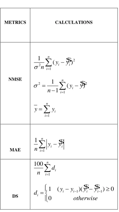
Network (BPN) as well as in Support Vector Machines (SVMs).To find the performances we have calculated 3 type of performance indicators which are Normalized Mean Square Error (NMSE), Mean Absolute Error (MAE) and Directional Symmetry (DS). The mean absolute error (MAE) is a quantity used to measure how close forecasts or predictions are to the eventual outcomes. The mean absolute error is a common measure of forecast error in time series analysis. NMSE and MAE are the measures of the deviation between the actual and predicted values. Their calculations have been given in Table 4. The above table shows the calculated error according to the data taken from BANK NIFTY and the 12 banks under BANK NIFTY using both Back Propagation Neural Network and Support Vector Machines .From table 4 we calculate the three types of performance indicators for both the models i.e. the BPNs and the SVMs by using the formulae of NMSE, MAE and DS. The smaller the values of NMSE and MAE, the closer are the predicted time series values to the actual values (a smaller value suggests a better predictor). DS provides an indication of the correctness of the predicted direction of RDP+5 given in the form of percentages (a larger value suggests a better predictor).

5. EXPERIMENTAL RESULTS AND

COMPARISON

5.1 Result 1

Figure 1: Plot for SISO Comparision

Figure 2: Plot for MISO Comparison

Figure 3: Plot for SISO Comparison (SVM)

SISO Comparision (ANN)

4000 4500 5000 5500 6000 6500 7000

1 7 13 19 25 31 37 43 49 55 61 67 73 79 85 91 97

TESTING TIME-->(In Days)

C LO S IN G P R IC E --> (I n R up e e s ) ACTUAL PREDICTED MISO Comparision(ANN) 4000 4500 5000 5500 6000 6500 7000

1 7 13 19 25 31 37 43 49 55 61 67 73 79 85 91 97

C LO S IN G P R IC E --> (I n R up e e s ) ACTUAL PREDICTED

SISO Comparision (SVM)

4000 4500 5000 5500 6000 6500 7000

1 7 13 19 25 31 37 43 49 55 61 67 73 79 85 91 97

C LO S IN G P R IC E --> (I n R U pe e s ) ACTUAL PREDICTED

METRICS CALCULATIONS

NMSE

$

2 2 1

1 (

)

n i i i

y

n









$

2 2 1

1 (

)

1

n i i

y

n









1 n i i

y





MAE

$

1

n i i i

y

n







DS 1

100

n i i

d

n





$ $

1 1

1 (

)(

)

0

i i i i

i

y

(5)

[image:5.595.319.550.74.175.2]

Figure 4: Plot for MISO Comparison (SVM)

Figure 5: Comparisons between ANN (MISO and SISO) and SVM (MISO and SISO) with Actual Closing

[image:5.595.56.290.78.204.2]

The above figure shows the graph plotted between the actual data and the data collected from neural network (Multiple input single output and single input with single output) and support vector machines (multiple input single output and single input with single output) of 100 day time series.

5.2 Result 2

Figure 6: Plot for 12 Bank Contribution Comparisons (BPN)

Figure 7: Plot for 12 Bank Contribution Comparisons (SVM)

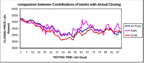
Figure 8: Comparison between Contributions of Banks with Actual Closing

The above figure shows the graph plotted between the actual closing data and the data collected from neural network and support vector machines of 100 day time series of 12 banks under Bank Nifty.

5.3Analysis of Results

It had been found that the NMSE for SISO in BPN and in SVMs is approximately same i.e 0.016 and 0.106 respectively. But the NMSE for MISO resulted is better in SVMs which is 0.0819.Same in case of DS in case of SISO both results are equal i.e 79 and in case of MISO SVMs provide better result i.e 73. The same result found for the 12 bank comparison which is been shown in result 2 and it had been found that the NMSE for ANN is more in predicting future volatility which is 0.742 but in case of SVM it is 0.429. We found the same result for the MAE where SVMs provide value 194.8331 where as BPN provides 233.567 and in case of DS also SVMs predicts better i.e 61 whereas BPN value is 57 . So from this we can conclude that SVMs predicts better.

6. ACKNOWLEDGMENTS

The authors thank the referees for the suggestions which improved the presentation of the paper.

7. REFERENCES

[1] L.J. Cao and Francis E. H. Tay, IEEE TRANSACTIONS ON NEURAL NETWORKS, VOL.14, NO.6, NOVEMBER 2003 Fröhlich, B. and Plate J. 2000,Support Vector Machines With Adaptive Parameters in Financial Time Series Forecasting. [2] Jibendu Kumar Mantri,Dr P.Gahan,B.B Nayak, ,Jibendu

Kumar Mantri et al./International journal of engeneering science and technology vol2(5).2010.1451-1460, Artificial Neural Networks-An application to stock market volatility .

[3] Y. Bao, Y. Lu, and J. Zhang, AIMSA 2004, LNAI 3192, pp. 295–303, 2004.© Springer-Verlag Berlin Heidelberg 2004, Department of Management Science & information System, Huazhong University of Science and Technology, China. C. Bussler and D. Fensel (Eds.). Forecasting Stock Price by SVMs Regression,

[4] E. Hajizadeh a, A. Seifi a,, M.H. Fazel Zarandi a, I.B. Turksen, 39 (2012) 431–436. 0957-4174/$ - see front matter _ 2011 Elsevier Ltd, Francis X. Diebold, Torben G. Andersen,Tim Bollerslev,P eter F. Christoffersen.Expert Systems with Applications. A

MISO Comparision (SVM)

4000 4500 5000 5500 6000 6500 7000

1 7 13 19 25 31 37 43 49 55 61 67 73 79 85 91 97

C LO S IN G P R IC E --> (I n R up e e s ) ACTUAL PREDICTED

Comparisons between ANN (MISO and SISO) and SVM (MISO and SISO)with Actual Closing

5000 5200 5400 5600 5800 6000 6200 6400

1 8 15 22 29 36 43 50 57 64 71 78 85 92 99

C LO S IN G P R IC E --> (I n R up e e s ) ACTUAL CLOSING SISO ANN MISO ANN SISO SVM MISO SVM

12 Bank Contribution Comparision(ANN)

3000 3500 4000 4500 5000 5500 6000

1 7 13 19 25 31 37 43 49 55 61 67 73 79 85 91 97

C LO S IN G P R IC E --> (I n R up e e s ) PREDICTED ACTUAL

12 Bank Contribution Comparision(SVM)

3000 3500 4000 4500 5000 5500 6000

1 7 13 19 25 31 37 43 49 55 61 67 73 79 85 91 97

TESTING TIME -->(In Days)

C LO S IN G P R IC E --> (I n R up e e s ) PREDICTED ACTUAL

comparison between Contributions of banks with Actual Closing

3000 3500 4000 4500 5000 5500 6000

1 7 13 19 25 31 37 43 49 55 61 67 73 79 85 91 97

[image:5.595.55.289.436.542.2] [image:5.595.58.293.594.697.2]

(6)

hybrid modeling approach for forecasting the volatility of S&P 500 index return

[5] Pei-Chann Chang, Di-di Wang, Chang-le Zhou, , Department of Information Management, Yuan Ze University, Taoyuan 32026, Taiwan Cognitive Science Department, Fujian Key Laboratory of Mind, Art and Computation, Xiamen University, Xiamen 361005, China. Expert Systems with Applications 39 (2012) 611– 620. 0957-4174/$ - see front matter _ 2011 Elsevier Ltd. A NOVEL MODEL BY EVOLVING PARTIALLY CONNECTED NEURAL NETWORK FOR STOCK PRICETREND FORECASTING.

[6] Anupam Tarsauliya, Shoureya Kant, Rahul Kala, Ritu Tiwari, Anupam Shukla, IIITM, walior, International journal of computer applications Volume 9- No.5, November-2010, ANALYSIS OF ARTIFICIAL NEURAL NETWORK FOR FINANCIAL TIME SERIES FORECASTING

[7] NSE of India Ltd., 2012, Available at: http://www.nseindia.com