http://dx.doi.org/10.4236/ojs.2014.45038
Random Route and Quota Sampling:
Do They Offer Any Advantage over
Probably Sampling Methods?
Vidal Díaz de Rada1, Valentín Martínez Martín2
1Departamento de Sociología, Public University of Navarre, Pamplona, Spain 2Centro de Investigaciones Sociológicas, Madrid, Spain
Email: [email protected], [email protected]
Received 28 May 2014; revised 2 July 2014; accepted 14 July 2014
Copyright © 2014 by authors and Scientific Research Publishing Inc.
This work is licensed under the Creative Commons Attribution International License (CC BY).
http://creativecommons.org/licenses/by/4.0/
Abstract
The aim of this paper is to compare sample quality across two probability samples and one that uses probabilistic cluster sampling combined with random route and quota sampling within the selected clusters in order to define the ultimate survey units. All of them use the face-to-face in-terview as the survey procedure. The hypothesis to be tested is that it is possible to achieve the same degree of representativeness using a combination of random route sampling and quota sampling (with substitution) as it can be achieved by means of household sampling (without subs-titution) based on the municipal register of inhabitants. We have found such marked differences in the age and gender distribution of the probability sampling, where the deviations exceed 6%. A different picture emerges when it comes to comparing the employment variables, where the quota sampling overestimates the economic activity rate (2.5%) and the unemployment rate (8%) and underestimates the employment rate (3.46%).
Keywords
Sampling Methods, Random Sampling, Multistage Cluster Sampling, Random Route Method, Quota Sampling
1. Introduction
the criticism focuses on its non-probability nature (which precludes the possibility of calculating sampling error), and the heavy influence of the interviewer in the choice of ultimate respondent.
Nevertheless, non-probability sampling methods remain among those commonly used by the majority of pri-vate opinion poll and market research companies [7] [8]; among others, whose predominant approach is quota sampling within households previously selected by the random methods [9]. Without denying the issues raised, the research sector has responded to the above mentioned criticism, which emanates mainly from academics and statisticians [3] [10], by claiming that these samples “work”, and, in fact, sometimes deliver better results than those obtained via strictly random sampling methods [5] [8].
The aim of this paper is to compare sample quality and response to the survey across two probability samples based on the municipal register of inhabitants and one that uses probabilistic cluster sampling combined with random route and quota sampling within the selected clusters in order to define the ultimate survey units. All of them use the face-to-face interview as the survey procedure. The hypothesis to be tested is that it is possible to achieve the same degree of representativeness using a combination of random route sampling and quota sam-pling (with substitution) as it can be achieved by means of household samsam-pling (without substitution) based on the municipal register of inhabitants. According to Bauer [9] “there are few studies focus on to assess the quality of random route samples”, and this one adds the use of selection with quota methods inside home.
The paper is organized into 5 sections. The introduction of the research topic is followed by the presentation of the data sources, with a brief indication of their differences and similarities. The three surveys are then com-pared, taking into account the distribution by age, sex, education and four employment variables (economic ac-tivity ratio, rate of unemployment, rate of employment and employment status). The discussion and conclusion sections are followed by the references used.
2. Data Sources
The two probability samples considered correspond to the European Social Survey (ESS) round 5, conducted in 2011, and the ISSP II Environmental Survey,which was carried out in 2010 by the Centro de Investigaciones Sociológicas—CIS, that is, the Spanish Sociological Research Centre, under an agreement signed with the ISSP (CIS survey number 2837). These two are compared with the sample used for the 2010 Health Barometer (henceforth HB) (CIS survey number 2850) where households are randomly drawn from census districts and respondents are selected within households using gender and age quotas. The next section presents the meth-odological details of these three samples.
2.1. European Social Survey (ESS)
The target universe is the population aged 15 years and over and resident in the main home in the whole of Spain (including Ceuta and Melilla), irrespective of nationality [11] [12]. The sampling frame is the municipal register. The universe is stratified by 17 autonomous regions and four municipal size categories: fewer than 10.001 inhabitants, 10.001 to 50.000 inhabitants, 50.001 to 100.00 inhabitants, and over 100.000 inhabitants
[13].
Since 2004 (the year of the second round) this survey has used two-stage cluster sampling from census dis-tricts with probability proportional to the size of the universe (resident population over the age of 15), taking 6 or 7 individuals from each district; 6 from smaller municipalities (<50,001 residents) and 7 from larger munici-palities (>50,000 residents) [11]. Respondents are drawn from lists taken from the May 2010 Municipal Register of inhabitants and supplied by the National Institute of Statistics (INE). The fieldwork was undertaken between April 11 and July 31, 2011 by 66 interviewers and 22 provincial coordinators.
2.2. ISSP (II) Environment Survey, CIS, Survey Number 2837
The universe for these surveys is all Spanish residents, of either sex, aged 18 and over, based on the 2009 mu-nicipal register sampling framework which has the same stratification as the European Social Survey, except that it has 7 municipal size categories: <2001 inhabitants; 2001 - 10,000; 10,001 - 50,000; 50,001 - 100,000; 100,001 - 400,000; 400,001 - 1,000,000, and >1,000,000 inhabitants. As in the ESS, it uses two-stage cluster sampling drawn from municipal registers with probability proportional to size, followed by a systematic selec-tion of individuals from households in each secselec-tion.
This survey is based on face-to-face interviews conducted in participants’ homes over the period May 13 to July 24, 2010. Of 4000 sample persons, 2560 were achieved, giving a participation rate of 64.5% after excluding 31 non-eligible subjects [16]. For a confidence level of 95.5% (two sigmas), and P = Q, the sampling error is ±1.98% for the sample as a whole. As in the ESS, refusals that persist after four visits to the household are not replaced.
Despite the similarity of the participation rates (66% for the ESS and 64% the Environment ISSP), the use of fewer techniques to ensure the participation of the more reluctant sample members in the second of these sur-veys explains the marked differential in number of non-contacts: 84 and 811 (3% and 20% of all attempted con-tacts), respectively.
2.3. Health Barometer 2010, CIS Survey 2850
The universe for the Health Barometeris the resident population aged 18 and over, stratified by autonomous re-gions, and 7 municipal size categories (<2001 inhabitants; 2001 - 10,000; 10,001 - 50,000; 50,001 - 100,000; 100,001 - 400,000; 400,001 - 1,000,000, and >1,000,000 inhabitants). Three nationally-representative subsam-ples of 2600 respondents were taken and interviewed in March, June, and the period October to November, us-ing multi-staged cluster samplus-ing, where the primary units (municipalities), and secondary units (census districts) were selected with probability proportional to size (numbers of residents aged 18 and over) [17]. The aggregate sample of 7750 questionnaires has a sampling error of ±1.13% for the sample as a whole, assuming simple ran-dom sampling, for a confidence level of 95.5% (two sigmas), and P = Q [18].
Households were randomly drawn from every other apartment building in each census district, using gender and age quotas for the selection of the ultimate respondent (household member) [17]. When the household con-tained more than one eligible interviewee, the youngest of these was selected for interview [19]. Whenever the interviewer was unable to conduct the interview in the appointed place (non-contact, refusal, etc.), the sample unit is replaced according to the standards laid out in the document General standards for correct sampling, which states that, “when an interview is not possible at the first contact, the interviewer can try next door” [19], that is, in the first household of the following segment (group of six households). In the case of apartment buildings, where no interview can be achieved, this address is replaced with the one next to it [19]. These pro-cedural methods explain why it was necessary to contact 161,395 households in order to achieve 7750 inter-views, which represents an average of 20.8 contacts per interview.
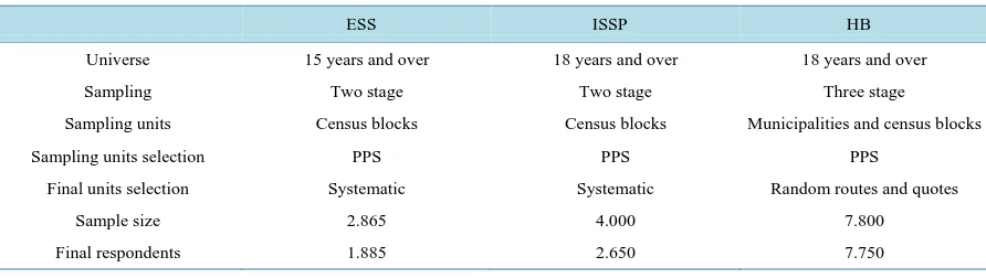
Summing up, let us note that all three surveys stratify by autonomous region and municipal size, the only dif-ference being that the ESS uses fewer strata (seeTable 1). The data are collected by means of face to face inter-views, using multi-stage (two-stage in the probability samplings, and multi-stage in the case of the HB) cluster samples drawn from municipal register data stratified by municipal size. It is from this point onwards that the differences between the three surveys begin. The HB uses a combined route/quota sampling procedure, whereas the ESS and the ISSP take random samples from lists of individuals. In addition, the ESS uses a wide range of resources to encourage participation (letters of presentation, re-contacts, refusal conversion techniques, produc-tivity-linked remuneration of interviewers, etc.), and the ISSP uses a letter of presentation, and four re-contacts. Another key difference is that the HB uses non-contact replacement, while the other two do not (seeTable 1).
3. Distribution Comparison
Table 1. Differences between those three sampling methods.
ESS ISSP HB
Universe 15 years and over 18 years and over 18 years and over
Sampling Two stage Two stage Three stage
Sampling units Census blocks Census blocks Municipalities and census blocks
Sampling units selection PPS PPS PPS
Final units selection Systematic Systematic Random routes and quotes
Sample size 2.865 4.000 7.800
Final respondents 1.885 2.650 7.750
Source: [13] [16] [18].
It would be interesting to extend the comparison to other highly relevant variables, such as educational at-tainment, and the economic activity ratio, about which there is no current data for the survey universe. There is, however, a source of data that is highly representative of the Spanish population. This is the Economically Ac-tive Population Survey (hence forth EAPS), which gathers and publishes statistics that are essential for an un-derstanding of the human side of the nation’s economic activity, with the primary objective of assessing the de-gree of economic activity and other related issues among the population [20]. It is the largest household survey in terms of sample size, workforce size, and cost.
As a result of the large size of the sample used for the EAPS, and in view of its particular design characteris-tics, it can be considered a source of data that are very similar to real Spanish population data. In addition, the EAPS also provides data on the economic activity ratio, the majority gender differentiated. For a discussion of the comparability of the two surveys, see Díaz de Rada and Núñez Villuendas [21]. This enables the comparison to include four of the most relevant socio-political research variables: age by gender, educational attainment by gender, and employment rate by gender.
Our analysis looks at the gender distributions rather than the marginal distributions of the variables of interest. The use of jointed distributions will enable us to detect differences in some variable frequencies that would go undetected if we were to use marginal distributions, where there is a possibility of cross-segment compensation. (In the first part ofTable 2, for example, if we were working with the marginal age distribution, the 55 to 64 age bracket would show a 0.45% negative deviation from the municipal register data; while the gender breakdown shows males to be under-represented by 0.67% and females to be over-represented by 0.21%. This enables us to attribute the observed deviation in that age bracket to males). These variables are examined separately in the following sections.
3.1. Age and Gender Comparisons
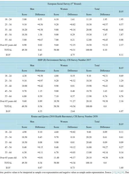
Table 2shows a comparison between the age distribution data from each survey and the sampling frame. Since the ESS used the 2010 municipal register and the fieldwork was conducted in 2011, the displayed age distribu-tion is for the populadistribu-tion in 2011. The discrepancy between the number of cases shown in Table 2 and the number mentioned in the sample design described above is due partly to the removal of under-eighteen year olds and Ceuta and Melilla residents and partly to the weighting of the data.
These points aside, the difference with the universe is just over 8 points, due mainly to the under-estimation by 2.33% of the population over the age of 64 years. It is also possible to observe over-estimation of the young-est population group and those in the 45 - 54 age bracket; as has been observed in every round of the survey up to the present [11]. The gender-differentiated analysis reveals slightly higher male representation. Males be-tween the ages of 45 and 54 are over-represented by 1.58%, while those in the 55 - 64 and 25 - 44 age brackets are under-represented. Females in the youngest age bracket are over-represented by 1.6%, and those in the over 65 age bracket are under-represented by more than 2%.
Table 2. Sample vs. universe comparison of age and gender distributions. Vertical percentages and differences between magnitudes (sample estimate minus universe).
European Social Survey (5th Round)
Men Women Total
SAV
Score Difference Score Difference Score Difference
18 - 24 5.00 0.33 6.10 1.61 11.10 1.95 1.95
25 - 34 9.10 −0.56 9.20 −0.02 18.30 −0.57 0.57
35 - 44 10.20 −0.30 9.80 −0.16 20.00 −0.46 0.46
45 - 54 10.30 1.58 9.00 0.29 19.30 1.87 1.87
55 - 64 5.80 −0.67 7.00 0.21 12.80 −0.45 0.88
Over 65 years old 8.90 0.02 9.60 −2.35 18.50 −2.33 2.37
TOTAL 49.30 0.41 50.80 −0.31 100.00 0.10
SAV 3.45 4.75 8.11
ISSP (II) Environment Survey, CIS Survey Number 2837
Men Women Total
SAV
Score Difference Score Difference Score Difference
18 - 24 4.30 −0.50 4.80 0.19 9.10 −0.31 0.69
25 - 34 9.10 −0.97 9.20 −0.32 18.30 −1.29 1.29
35 - 44 10.00 −0.42 9.90 0.01 19.90 −0.41 0.44
45 - 54 9.70 1.15 9.00 0.48 18.70 1.63 1.63
55 - 64 6.80 0.39 7.10 0.37 13.90 0.76 0.76
Over 65 years old 9.60 0.89 10.50 −1.27 20.10 −0.38 2.16
TOTAL 49.50 0.54 50.50 −0.54 100.00 0.0
SAV 4.33 2.64 6.97
Routes and Quotes (2010 Health Barometer), CIS Survey Number 2850
Men Women Total
SAV
Score Difference Score Difference Score Difference
18 - 24 4.90 0.10 4.60 −0.02 9.60 0.09 0.11
25 - 34 10.50 0.43 9.70 0.18 20.20 0.61 0.61
35 - 44 10.50 0.08 9.90 0.01 20.40 0.09 0.09
45 - 54 8.40 −0.15 8.40 −0.12 16.80 −0.27 0.27
55 - 64 6.30 −0.11 6.70 −0.03 13.00 −0.14 0.14
Over 65 years old 8.70 −0.01 11.40 −0.37 20.10 −0.38 0.38
TOTAL 49.30 0.34 50.80 −0.34 100.10 0.0
SAV 0.87 0.73 1.60
These three subgroups account for 68.4% of the age- and gender-related deviation.
The “ISSP II Environment Survey” uses the Municipal Register for 2009 (CIS, 2010) as its sample frame and carries out the fieldwork in July 2010, which produces a similar situation to that of the preceding case. That is, the age distribution shown inTable 2 is for the 2010 population. The differences with respect to the Municipal Register decrease to 6.97 points, and the under-representation of over 65-year-old (especially females) accounts for most of this deviation. The next most noteworthy feature is the over-estimation of the 45 - 54 age bracket.
The distribution by gender shows that the sample does not adequately represent males. The 45 - 54 male age bracket is overestimated by 1.15%, and younger men are underestimated overall and to a slightly higher degree in the 25 - 34 age bracket (0.50%, 0.97% and 0.42%). The main difference in the case of the females lies in the under-estimation of the over 65 age group, and the over-estimation of the 45 - 54 age group.
The subgroups that contribute most to the observed deviations are older women and men between the ages of 45 and 54. These two subgroups account for 34.7% of the observed differences, with the percentage deviation explained increasing to 48.6% when the male 25 - 34 age bracket is included.
When compared, the HB and the January 1, 2010 revision of the Municipal Register show strong similarity in all age brackets, except the 25 to 34 age bracket, which is over-represented by 0.61%. From that point onwards, we find slight but increasing under-representation, which reaches a level of 0.38% in the oldest age bracket. The 35 to 44 age bracket is the best represented. Differentiating by gender, we find the most poorly represented group to be that of males between the ages of 25 and 34, followed by older females. In both cases, the difference is less than 1%, and is therefore attributable to sampling error (±1.13%). Taken together, these two groups ex-plain half of the total deviation, which—it should be noted—is 1.60%.
It appears logical that the quota-based sample should display fewer differences in the age and gender distribu-tions than samples obtained by other procedures, which might make this comparison appear spurious. However, we consider it justifiable by the fact that interviewers are authorized to replace a respondent from one quota with another (of the same sex) from the adjacent quota when contact proves difficult. Despite the fact that detailed analysis of the fieldwork records shows that contact difficulties involved mainly young people and were slightly more frequent in the case of females, they have no significant impact on the representativeness of the age and gender distributions.
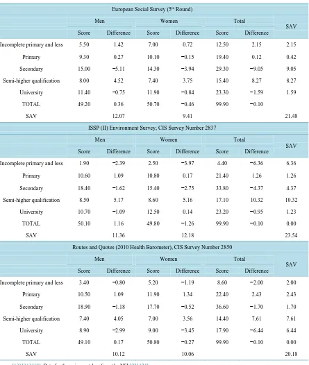
3.2. Differences in the Educational Attainment Distribution
The responses to the educational attainment questions were recoded to align them with the EAPS categorization. As can be seen in the first part ofTable 3, the deviation in the ESS arises mainly from under-estimation in the secondary education category (−9.05%), strong over-representation in the semi-higher qualification category (8.27%), and somewhat less marked over-representation in the incomplete primary and less category (2.15%). The absolute differences of the male and female secondary education categories, divided by total standard de-viation (21.48%), show that they account for 42.12% of all the dede-viation in the table.
The ISSP II Environment Survey over-estimates the semi-higher qualification category (10.32%) and under- estimates the incomplete primary and less category (−6.36%), the deviation being greater in the female
sub-category (−3.97%). The subcategories that contribute most to the total deviation are the semi-higher qualifica-tion category and the female incomplete primary and less category, which, together, account for 60.7% (and 70.9% when the male incomplete primary and less category is included). Note that this survey provides a better representation of men but a poorer representation of women, in complete contrast to the ESS. In sum, the marked differences in educational attainment found in the two probability samplings showed a sum of absolute differences of 21.48 and 23.54 points, respectively.
The data compiled by the HB (using random route and quotas) are somewhat better, since none of the differ-ences across the table enter double figures. There is 7.61% over-estimation in the semi-higher qualification
Table 3. Sample vs. universe comparison of the education distribution by gender. Vertical percentages and differences be-tween magnitudes (sample estimate minus universe).
European Social Survey (5th Round)
Men Women Total
SAV
Score Difference Score Difference Score Difference
Incomplete primary and less 5.50 1.42 7.00 0.72 12.50 2.15 2.15
Primary 9.30 0.27 10.10 −0.15 19.40 0.12 0.42
Secondary 15.00 −5.11 14.30 −3.94 29.30 −9.05 9.05
Semi-higher qualification 8.00 4.52 7.40 3.75 15.40 8.27 8.27
University 11.40 −0.75 11.90 −0.84 23.30 −1.59 1.59
TOTAL 49.20 0.36 50.70 −0.46 99.90 −0.10
SAV 12.07 9.41 21.48
ISSP (II) Environment Survey, CIS Survey Number 2837
Men Women Total
SAV
Score Difference Score Difference Score Difference
Incomplete primary and less 1.90 −2.39 2.50 −3.97 4.40 −6.36 6.36
Primary 10.60 1.09 10.80 0.17 21.40 1.26 1.26
Secondary 18.40 −1.62 15.40 −2.75 33.80 −4.37 4.37
Semi-higher qualification 8.50 5.17 8.60 5.16 17.10 10.32 10.32
University 10.70 −1.09 12.50 0.14 23.20 −0.95 1.23
TOTAL 50.10 1.16 49.80 −1.26 99.90 −0.10 0.00
SAV 11.36 12.18 23.54
Routes and Quotes (2010 Health Barometer), CIS Survey Number 2850
Men Women Total
SAV
Score Difference Score Difference Score Difference
Incomplete primary and less 3.40 −0.80 5.20 −1.19 8.60 −2.00 2.00
Primary 10.50 1.09 11.90 1.34 22.40 2.43 2.43
Secondary 18.90 −1.18 17.70 −0.52 36.60 −1.70 1.70
Semi-higher qualification 7.40 4.05 7.00 3.56 14.40 7.61 7.61
University 8.90 −2.99 9.00 −3.45 17.90 −6.44 6.44
TOTAL 49.10 0.17 50.80 −0.27 99.90 −0.10 0.00
SAV 10.12 10.06 20.18
Source: [13] [16] [18]. Data for the universe taken from the NSI [23] [24].
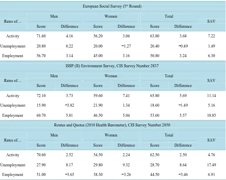
3.3. Sample vs. Universe Comparison of Employment Variables
distinguishes the economically active from the unemployed by purposely wording the questions. In other words, in the surveys considered in this paper, “unemployed” is an ascription that covers respondents who may, in fact, be non-active, that is, not part of the economically active population. This point will be discussed further at a later stage.
Table 4shows that the ESS over-estimates both the economic activity rate (particularly the male estimate) and the employment rate. The ESS unemployment rate estimate is, nevertheless, 0.49% lower than reported by the EAPS, which estimated female unemployment less accurately. It should be noted, however, that this is the lowest deviation found in any of the surveys considered, and that there is no observable change in the results when the population aged 16 to 17 and Ceuta and Melilla residents are included.
Wider deviation can be observed in all three estimates given by the ISSP II Environment Survey, whose eco-nomic activity and employment rates deviate from the EAPS by more than 5%. Differentiation by gender reveals the widest deviations to be the over-estimation of the female economic activity rate (7.41%) and the over-esti- mation of the male employment rate (3.73%). It is also possible to observe an under-estimation of the overall unemployment rate by 1.49%, and by double that amount in the male unemployment subgroup. The sum of ab-solute values (SAV) reveals deviations of more than 10 points in the economic activity and employment rates.
The HB over-estimates the economic activity and unemployment rates, the second of these by 8.64%, and the female unemployment subgroup by even more (9.32%). The sum of absolute values (SAV) of differences in the unemployment rate is 17.5 points, which is the widest observed deviation in this study, which also finds the overall employment rate to be under-estimated by 3.46%, and male employment by 3.65%.
Table 4. Sample vs. universe comparison of economic activity, unemployment and employments rates by gender. Vertical
percentages and differences between magnitudes (sample estimate minus universe).
European Social Survey (5th Round)
Rates of…
Men Women Total
SAV
Score Difference Score Difference Score Difference
Activity 71.60 4.16 56.20 3.06 63.80 3.68 7.22
Unemployment 20.80 0.22 20.00 −1.27 20.40 −0.49 1.49
Employment 56.70 3.14 45.00 3.16 50.80 3.24 6.30
ISSP (II) Environment Survey, CIS Survey Number 2837
Rates of…
Men Women Total
SAV
Score Difference Score Difference Score Difference
Activity 72.10 3.73 59.60 7.41 65.80 5.69 11.14
Unemployment 15.90 −3.82 21.90 1.34 18.60 −1.49 5.16
Employment 60.70 5.81 46.50 5.04 53.60 5.57 10.85
Routes and Quotes (2010 Health Barometer), CIS Survey Number 2850
Rates of…
Men Women Total
SAV
Score Difference Score Difference Score Difference
Activity 70.60 2.52 54.50 2.24 62.50 2.50 4.76
Unemployment 27.90 8.17 29.80 9.32 28.70 8.64 17.49
Employment 51.00 −3.65 38.30 −3.26 44.50 −3.46 6.91
4. Discussion
It comes as a surprise to find such marked differences in the age and gender distribution of the probability sam-pling, where the joint deviation exceed 6 points, and can, therefore, in no way be explained by sampling error. The most noteworthy discrepancies are those that appear between the two probability samplings—which, as al-ready noted, use a similar sampling design—and can, therefore, only be attributed to the techniques used by the ESS to increase survey participation. Re-contacts and refusal conversion techniques enabled the ESS—in the third round (2006)—to retrieve 18.3% and 6.3% of the sample, respectively. Differences in the successful rep-resentation of the universe can be explained by the specific features of these two respondent groups [27].
The quality of the HB data is superior to that achieved by the two probability sampling-based surveys, due to the use of age and gender quotas. These require the interviewers to seek out individuals with given characteris-tics, with the result that the sample matches the universe because of the nature of the quota selection policy. In light of these considerations, quota replacements, by which interviewers are permitted to substitute a non-con- tact with an individual from an adjacent quota in either direction, are offset by replacements made by other in-terviewers in the opposite direction, and can, therefore, be classed as errors that cancel each other out. Given that the sample is defined by the age and gender distribution in the universe, age and gender quotas serve little purpose, except to confirm that age and gender are not strongly associated with other variables, such as the eco-nomic activity rate. This casts some doubt on the usefulness of age and gender data for quota sampling.
The range of differences that appear in the probability samplings is situated between 10.32 points in the esti-mation of semi-higher qualification category figures in the ISSP II Environment, and 0.12 points in the primary education figures obtained by the ESS. These two surveys present deviations of 23.54 and 21.48 points, respec-tively. The HB, in contrast, reflects educational attainment in the population slightly better (20.18 points). This could be due to lower age dispersion, since there is a very close link between age and educational attainment.
A completely different picture emerges when it comes to comparing the employment variables, particularly with respect to the employment, economic activity, and unemployment rates. The ESS over-estimates the eco-nomic activity and employment rates by more than 3 points, and more than 4 points in the male subcategory, while the Environment Survey reports even higher rates, particularly in the female activity (7.41%) and in the male employment where the deviations reach the 5.81%. The HB overestimates the economic activity rate by 2.5% and the unemployment rate by 8.64% (9.3% in the case of women), and under-estimates the employment rate by 3.46%.
Two important issues underlie these differences. The first has to do with the different universes under consid-eration, the population over the age of 15 in the EAPS and the population over the age of 18 in the HB. More significantly, from our point of view, the survey designed for the HB—as noted previously—recommends inter-viewers to substitute addresses where there is no reply with the one next door. Calling at one household after another (up to 20.8 contacts) results in the replacement both of households where there is no reply—because the occupants are at work or absent for other reasons—and those that are empty–because they are second homes or (to a lesser degree) false entries in the municipal register—with households whose occupants are at home when the interviewer calls. Given that the employed spend less time at home than the unemployed, the probability of not being at home when the interviewer calls is higher among the employed than among the unemployed. In our opinion, this is the reason for the higher rate of unemployed found by the HB (and similar surveys).
This could account for the marked over-estimation of the unemployment rate. The large number of unem-ployed also explains the higher economic activity ratio, which is calculated as the active population (emunem-ployed and unemployed) over the population as a whole.
5. Conclusion
Thus, in summary, random route and quota samples provide a better representation of the age and educational attainment distributions, but over-estimate the figures for the unemployment variable, which the probability samplings estimate more accurately. The CIS, however, which uses random route and quota sampling with sub-stitution methods, obtains more representative samples than other surveys of its type conducted in Spain [29].
Authors and Affiliations
Vidal Díaz de Rada Igúzquiza, Public University of Navarre, Dpto de Sociología, 31006 Pamplona-Spain, Valentín Martínez Martín, Centro de Investigaciones Sociológicas, Montalban 8, 28014 Madrid-Spain.
Acknowledgements
This work was supported by Ministerio de Economía y Competitividad (Government of Spain) (grant number CSO2012-34257).
References
[1] Marsh, C. and Scarbrough, E. (1990) Testing Nine Hypotheses about Quota Sampling. Journal of the Market Research Society, 32, 485-506.
[2] Kish, L. (1965) Survey Sampling. Wiley, New York.
[3] Kish, L. (1998) On Quota Sampling. Working Paper, Universidad de Michigan. http://www.websm.org/uploadi/editor/1132389572kish.doc
[4] Kish, L. (1998) Quota Sampling: Old plus New Thought. Working Paper, Universidad de Michigan, Unpublished. [5] Sudman, S. and Blair, E. (1999) Sampling in the Twenty-First Century. Journal of the Academy of Marketing Science,
27, 269-277.
[6] Armate, M. (2004) La introducción en Francia de los métodos de sondeo aleatorio. Empiria, 8, 70-80.
[7] Rothman, J. and Dawn, M. (1989) Statisticians Can Be Creative Too. Journal of the Market Research Society, 31, 456- 466.
[8] Taylor, H., Harris, L. and Associated (1995) Horses for Courses: How Survey Firms in Different Countries Measure Public Opinion with Very Different Methods. Journal of the Market Research Society, 37, 211-219.
[9] Bauer, J.J. (2014) Selection Errors of Random Route Samples. Sociological Methods & Research. http://smr.sagepub.com/content/early/2014/02/24/0049124114521150
[10] Burton, D. (2000) Research Training for Social Scientist. Sage, London.
[11] Cuxart, A. and Riba, C. (2009) Mejorando a partir de la experiencia: La implementación de la tercera ola de a ESE en España. Revista Española de Investigaciones Sociológicas, 125, 147-165.
[12] Stoop, I., Billiet, J., Koch, A. and Fitzgerald, R. (2010) Improving Survey Response: Lessons Learned from the Euro-pean Social Survey. Wiley, Chichester.
[13] Spanish National Team European Social Survey (2011) Documentation of the Spanish Sampling Procedure 2010. http://www.upf.edu/ess/datos/quinta-ed.html
[14] National Institute of Statistics (INE) (2010) Continuous Municipal Register Statistics, Definitive Results 2010. http://www.ine.es/jaxi/menu.do?type=pcaxis&path=%2Ft20%2Fe245&file=inebase&L=1
[15] Spanish National Team European Social Survey and Metroscopia (2011) Final Field Report of the 4th Round of ESS. http://www.upf.edu/ess/datos/quinta-ed.html#infadicional
[16] Centro de Investigaciones Sociológicas (CIS) (2010) Medio ambiente (II) ISSP. CIS Survey No. 2837. [17] Martín, V.C.M. (2004) Diseño de encuestas de opinión. Rama, Madrid.
[18] CIS (2010) Barómetro Sanitario. CIS Survey No. 2850.
[19] CIS (2010) Normas generales para la correcta aplicación de la muestra. CIS, Madrid.
[20] National Institute of Statistics (INE) Economically Active Population Survey, Methodology. http://www.ine.es/en/inebaseDYN/epa30308/epa_metodologia_en.htm
[21] De Rada, V.D. and Villuendas, A.N. (2008) Estudio de las incidencias en la investigación con encuesta. El caso de los barómetros del CIS, CIS, Madrid.
[23] National Institute of Statistics (INE) (2010) Economically Active Population Survey, National Results 2010: Activity and Unemployment Rate, Sex and Age Group.
[24] National Institute of Statistics (INE) (2011) Economically Active Population Survey, National Results 2011: Activity and Unemployment Rate, Sex and Age Group.
[25] National Institute of Statistics (INE) (2010) Economically Active Population Survey, National Results 2010: Popula- tion Aged 16 Years Old and Over by Sector of the Level of Education Attained, Sex and Age Group.
[26] National Institute of Statistics (INE) (2011) Economically Active Population Survey, National Results 2011: Popula-tion Aged 16 Years Old and Over by Sector of the Level of EducaPopula-tion Attained, Sex and Age Group.
[27] Riba, C., Torcal, M. and Morales, L. (2010) Estrategias para aumentar la tasa de respuesta y los resultados de la Encu- esta Social Europea en España. Revista Internacional de Sociología, 68, 603-635.
http://dx.doi.org/10.3989/ris.2008.12.17
[28] Durán Heras, M.Á. (2012) El Trabajo no remunerado en la economía global. BBVA Fundation, Bilbao.